Download
1 / 57
570 likes | 576 Views
Learn how to apply iterative repair and iterative improvement to constraint satisfaction problems, including the Traveling Salesman Problem. Understand the min-conflict strategy, local minima problem, and other methods like simulated annealing and genetic algorithms.

E N D
Searching by Constraint(Continued) CMSC 25000 Artificial Intelligence January 29, 2008
Incremental Repair • Start with initial complete assignment • Use greedy approach • Probably invalid - I.e. violates some constraints • Incrementally convert to valid solution • Use heuristic to replace value that violates • “min-conflict” strategy: • Change value to result in fewest constraint violations • Break ties randomly • Incorporate in local or backtracking hill-climber
Q2 Q4 Q1 Q3 Q2 Q4 Q1 Q3 Incremental Repair Q2 Q4 5 conflicts Q1 Q3 0 conflicts 2 conflicts
Question • How would we apply iterative repair to Traveling Salesman Problem?
Iterative Improvement • Alternate formulation of CSP • Rather than DFS through partial assignments • Start with some complete, valid assignment • Search for optimal assignment wrt some criterion • Example: Traveling Salesman Problem • Minimum length tour through cities, visiting each one once
Iterative Improvement Example • TSP • Start with some valid tour • E.g. find greedy solution • Make incremental change to tour • E.g. hill-climbing - take change that produces greatest improvement • Problem: Local minima • Solution: Randomize to search other parts of space • Other methods: Simulated annealing, Genetic alg’s
Min-Conflict Effectiveness • N-queens: Given initial random assignment, can solve in ~ O(n) • For n < 10^7 • GSAT (satisfiability) • Best (near linear in practice) solution uses min-conflict-type hill-climbing strategy • Adds randomization to escape local min • ~Linear seems true for most CSPs • Except for some range of ratios of constraints to variables • Avoids storage of assignment history (for BT)
Evolutionary Search Artificial Intelligence CMSC 25000 January 29, 2008
Agenda • Motivation: • Evolving a solution • Genetic Algorithms • Modelling search as evolution • Mutation • Crossover • Survival of the fittest • Survival of the most diverse • Conclusions
Motivation: Evolution • Evolution through natural selection • Individuals pass on traits to offspring • Individuals have different traits • Fittest individuals survive to produce more offspring • Over time, variation can accumulate • Leading to new species
Simulated Evolution • Evolving a solution • Begin with population of individuals • Individuals = candidate solutions ~chromosomes • Produce offspring with variation • Mutation: change features • Crossover: exchange features between individuals • Apply natural selection • Select “best” individuals to go on to next generation • Continue until satisfied with solution
Genetic Algorithms Applications • Search parameter space for optimal assignment • Not guaranteed to find optimal, but can approach • Classic optimization problems: • E.g. Travelling Salesman Problem • Program design (“Genetic Programming”) • Aircraft carrier landings
Genetic Algorithm Example • Cookie recipes (Winston, AI, 1993) • As evolving populations • Individual = batch of cookies • Quality: 0-9 • Chromosomes = 2 genes: 1 chromosome each • Flour Quantity, Sugar Quantity: 1-9 • Mutation: • Randomly select Flour/Sugar: +/- 1 [1-9] • Crossover: • Split 2 chromosomes & rejoin; keeping both
Fitness • Natural selection: Most fit survive • Fitness= Probability of survival to next gen • Question: How do we measure fitness? • “Standard method”: Relate fitness to quality • :0-1; :1-9: Chromosome Quality Fitness 1 4 3 1 1 2 1 1 4 3 2 1 0.4 0.3 0.2 0.1
GA Design Issues • Genetic design: • Identify sets of features = genes; Constraints? • Population: How many chromosomes? • Too few => inbreeding; Too many=>too slow • Mutation: How frequent? • Too few=>slow change; Too many=> wild • Crossover: Allowed? How selected? • Duplicates?
GA Design: Basic Cookie GA • Genetic design: • Identify sets of features: 2 genes: flour+sugar;1-9 • Population: How many chromosomes? • 1 initial, 4 max • Mutation: How frequent? • 1 gene randomly selected, randomly mutated • Crossover: Allowed? No • Duplicates? No • Survival: Standard method
Basic Cookie GA Results • Results are for 1000 random trials • Initial state: 1 1-1, quality 1 chromosome • On average, reaches max quality (9) in 16 generations • Best: max quality in 8 generations • Conclusion: • Low dimensionality search • Successful even without crossover
Basic Cookie GA+Crossover Results • Results are for 1000 random trials • Initial state: 1 1-1, quality 1 chromosome • On average, reaches max quality (9) in 14 generations • Conclusion: • Faster with crossover: combine good in each gene • Key: Global max achievable by maximizing each dimension independently - reduce dimensionality
1 2 3 4 5 4 3 2 1 2 0 0 0 0 0 0 0 2 3 0 0 0 0 0 0 0 3 4 0 0 7 8 7 0 0 4 5 0 0 8 9 8 0 0 5 4 0 0 7 8 7 0 0 4 3 0 0 0 0 0 0 0 3 2 0 0 0 0 0 0 0 2 1 2 3 4 5 4 3 2 1 Solving the Moat Problem • Problem: • No single step mutation can reach optimal values using standard fitness (quality=0 => probability=0) • Solution A: • Crossover can combine fit parents in EACH gene • However, still slow: 155 generations on average
Questions • How can we avoid the 0 quality problem? • How can we avoid local maxima?
Rethinking Fitness • Goal: Explicit bias to best • Remove implicit biases based on quality scale • Solution: Rank method • Ignore actual quality values except for ranking • Step 1: Rank candidates by quality • Step 2: Probability of selecting ith candidate, given that i-1 candidate not selected, is constant p. • Step 2b: Last candidate is selected if no other has been • Step 3: Select candidates using the probabilities
Rank Method Chromosome Quality Rank Std. Fitness Rank Fitness 1 4 1 3 1 2 5 2 7 5 4 3 2 1 0 1 2 3 4 5 0.4 0.3 0.2 0.1 0.0 0.667 0.222 0.074 0.025 0.012 Results: Average over 1000 random runs on Moat problem - 75 Generations (vs 155 for standard method) No 0 probability entries: Based on rank not absolute quality
Diversity • Diversity: • Degree to which chromosomes exhibit different genes • Rank & Standard methods look only at quality • Need diversity: escape local min, variety for crossover • “As good to be different as to be fit”
Rank-Space Method • Combines diversity and quality in fitness • Diversity measure: • Sum of inverse squared distances in genes • Diversity rank: Avoids inadvertent bias • Rank-space: • Sort on sum of diversity AND quality ranks • Best: lower left: high diversity & quality
Rank-Space Method W.r.t. highest ranked 5-1 Chromosome Q D D Rank Q Rank Comb Rank R-S Fitness 4 3 2 1 0 0.04 0.25 0.059 0.062 0.05 1 5 3 4 2 1 2 3 4 5 0.667 0.025 0.222 0.012 0.074 1 4 3 1 1 2 1 1 7 5 1 4 2 5 3 Diversity rank breaks ties After select others, sum distances to both Results: Average (Moat) 15 generations
GA’s and Local Maxima • Quality metrics only: • Susceptible to local max problems • Quality + Diversity: • Can populate all local maxima • Including global max • Key: Population must be large enough
GA Discussion • Similar to stochastic local beam search • Beam: Population size • Stochastic: selection & mutation • Local: Each generation from single previous • Key difference: Crossover – 2 sources! • Why crossover? • Schema: Partial local subsolutions • E.g. 2 halves of TSP tour
Question • Traveling Salesman Problem • CSP-style Iterative refinement • Genetic Algorithm • N-Queens • CSP-style Iterative refinement • Genetic Algorithm
Iterative Improvement Example • TSP • Start with some valid tour • E.g. find greedy solution • Make incremental change to tour • E.g. hill-climbing - take change that produces greatest improvement • Problem: Local minima • Solution: Randomize to search other parts of space • Other methods: Simulated annealing, Genetic alg’s
Machine Learning:Nearest Neighbor &Information Retrieval Search Artificial Intelligence CMSC 25000 January 29, 2008
Agenda • Machine learning: Introduction • Nearest neighbor techniques • Applications: • Credit rating • Text Classification • K-nn • Issues: • Distance, dimensions, & irrelevant attributes • Efficiency: • k-d trees, parallelism
Machine Learning • Learning: Acquiring a function, based on past inputs and values, from new inputs to values. • Learn concepts, classifications, values • Identify regularities in data
Machine Learning Examples • Pronunciation: • Spelling of word => sounds • Speech recognition: • Acoustic signals => sentences • Robot arm manipulation: • Target => torques • Credit rating: • Financial data => loan qualification
Complexity & Generalization • Goal: Predict values accurately on new inputs • Problem: • Train on sample data • Can make arbitrarily complex model to fit • BUT, will probably perform badly on NEW data • Strategy: • Limit complexity of model (e.g. degree of equ’n) • Split training and validation sets • Hold out data to check for overfitting
Nearest Neighbor • Memory- or case- based learning • Supervised method: Training • Record labeled instances and feature-value vectors • For each new, unlabeled instance • Identify “nearest” labeled instance • Assign same label • Consistency heuristic: Assume that a property is the same as that of the nearest reference case.
Nearest Neighbor Example • Credit Rating: • Classifier: Good / Poor • Features: • L = # late payments/yr; • R = Income/Expenses Name L R G/P A 0 1.2 G B 25 0.4 P C 5 0.7 G D 20 0.8 P E 30 0.85 P F 11 1.2 G G 7 1.15 G H 15 0.8 P
Nearest Neighbor Example Name L R G/P A 0 1.2 G A F B 25 0.4 P 1 G R E C 5 0.7 G H D C D 20 0.8 P E 30 0.85 P B F 11 1.2 G G 7 1.15 G 10 20 30 L H 15 0.8 P
Nearest Neighbor Example Name L R G/P I 6 1.15 G A F K J 22 0.45 P 1 I G ?? E K 15 1.2 D H R C J B Distance Measure: Sqrt ((L1-L2)^2 + [sqrt(10)*(R1-R2)]^2)) - Scaled distance 10 20 30 L
Nearest Neighbor Analysis • Problem: • Ambiguous labeling, Training Noise • Solution: • K-nearest neighbors • Not just single nearest instance • Compare to K nearest neighbors • Label according to majority of K • What should K be? • Often 3, can train as well
Matching Topics and Documents • Two main perspectives: • Pre-defined, fixed, finite topics: • “Text Classification” • Arbitrary topics, typically defined by statement of information need (aka query) • “Information Retrieval”
Vector Space Information Retrieval • Task: • Document collection • Query specifies information need: free text • Relevance judgments: 0/1 for all docs • Word evidence: Bag of words • No ordering information
Vector Space Model Tv Program Computer Two documents: computer program, tv program Query: computer program : matches 1 st doc: exact: distance=2 vs 0 educational program: matches both equally: distance=1
Vector Space Model • Represent documents and queries as • Vectors of term-based features • Features: tied to occurrence of terms in collection • E.g. • Solution 1: Binary features: t=1 if present, 0 otherwise • Similiarity: number of terms in common • Dot product
Vector Space Model II • Problem: Not all terms equally interesting • E.g. the vs dog vs Levow • Solution: Replace binary term features with weights • Document collection: term-by-document matrix • View as vector in multidimensional space • Nearby vectors are related • Normalize for vector length
Vector Similarity Computation • Similarity = Dot product • Normalization: • Normalize weights in advance • Normalize post-hoc
Term Weighting • “Aboutness” • To what degree is this term what document is about? • Within document measure • Term frequency (tf): # occurrences of t in doc j • “Specificity” • How surprised are you to see this term? • Collection frequency • Inverse document frequency (idf):
Term Selection & Formation • Selection: • Some terms are truly useless • Too frequent, no content • E.g. the, a, and,… • Stop words: ignore such terms altogether • Creation: • Too many surface forms for same concepts • E.g. inflections of words: verb conjugations, plural • Stem terms: treat all forms as same underlying
Efficient Implementations • Classification cost: • Find nearest neighbor: O(n) • Compute distance between unknown and all instances • Compare distances • Problematic for large data sets • Alternative: • Use binary search to reduce to O(log n)
Efficient Implementation: K-D Trees • Divide instances into sets based on features • Binary branching: E.g. > value • 2^d leaves with d split path = n • d= O(log n) • To split cases into sets, • If there is one element in the set, stop • Otherwise pick a feature to split on • Find average position of two middle objects on that dimension • Split remaining objects based on average position • Recursively split subsets