Download
1 / 27
270 likes | 369 Views
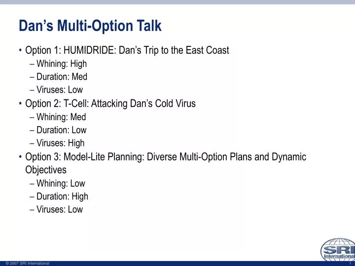
Dan’s Multi-Option Talk. Option 1: HUMIDRIDE: Dan’s Trip to the East Coast Whining: High Duration: Med Viruses: Low Option 2: T-Cell: Attacking Dan’s Cold Virus Whining: Med Duration: Low Viruses: High Option 3: Model-Lite Planning: Diverse Multi-Option Plans and Dynamic Objectives

E N D
Dan’s Multi-Option Talk • Option 1: HUMIDRIDE: Dan’s Trip to the East Coast • Whining: High • Duration: Med • Viruses: Low • Option 2: T-Cell: Attacking Dan’s Cold Virus • Whining: Med • Duration: Low • Viruses: High • Option 3: Model-Lite Planning: Diverse Multi-Option Plans and Dynamic Objectives • Whining: Low • Duration: High • Viruses: Low
Model-Lite Planning: Diverse Multi-Option Plans and Dynamic Objectives Daniel Bryce William Cushing Subbarao Kambhampati
Questions • When must the plan executor decide on their planning objective? • Before synthesis? • Traditional model • Before execution? • Similar to IR model: select plan from set of diverse, but relevant plans • During execution? • Multi-Option Plans (subsumes previous) • At all? • “Keep your options open” • Can the executor change their planning objective without replanning? • Can the executor start acting without committing to an objective?
Overview • Diverse Multi-Option Plans • Diversity • Representation • Connection to Conditional Plans • Execution • Synthesizing Multi-Option Plans • Example • Speed-ups • Analysis • Synthesis • Execution • Conclusion
Cost O2 O1 O2a O1a Diversity Duration Cab(PVD, Prov.) Fly(BOS,PVD) O1a Fly(SFO, BOS) Train(MP, SFO) Car(BOS,Prov.) O1 Cab(PVD, Prov.) Fly(BOS,PVD) O2a Fly(SFO, BOS) Shuttle(MP, SFO) O2 Car(BOS,Prov.) Diverse Multi-Option Plans • Each plan step presents several diverse choices • Option 1: Train(MP, SFO), Fly(SFO, BOS), Car(BOS, Prov.) • Option 1a: Train(MP, SFO), Fly(SFO, BOS), Fly(BOS, PVD), Cab(PVD, Prov.) • Option 2: Shuttle(MP, SFO), Fly(SFO, BOS), Car(BOS, Prov.) • Option2a: Shuttle(MP, SFO), Fly(SFO, BOS), Fly(BOS, PVD), Cab(PVD, Prov.) • Diversity is Reliant on Pareto Optimality • Each option is non-dominated • Diversity through Pareto Front w/ High Spread
Cab(PVD, Prov.) Fly(BOS,PVD) O1a Fly(SFO, BOS) Train(MP, SFO) Car(BOS,Prov.) O1 Cab(PVD, Prov.) Fly(BOS,PVD) O2a Fly(SFO, BOS) Shuttle(MP, SFO) O2 Car(BOS,Prov.) Dynamic Objectives • Multi-Options Plans are a type of Conditional Plan • Conditional on the user’s Objective Function • Allow the objective Function to change • Ensured that, irrespective of their obj. fn., will have non-dominated options
Option values Change at each step Cost Cost Cost O1 O1 O1a O1 O1a Duration Duration Duration Cost O2 O1 O2a O1a Duration Executing Multi-Option Plans Local action choice corresponds to multiple options Cab(PVD, Prov.) Fly(BOS,PVD) O1a Fly(SFO, BOS) Train(MP, SFO) Car(BOS,Prov.) O1 Cab(PVD, Prov.) Fly(BOS,PVD) O2a Fly(SFO, BOS) Shuttle(MP, SFO) O2 Car(BOS,Prov.)
Multi-Option Conditional Probabilistic Planning • (PO)MDP setting: (Belief) State Space Search • Stochastic Actions, Observations, Uncertain Initial State, Loops • Two Objectives: Expected Plan Cost, Probability of Plan Success • Traditional Reward functions are linear combination of above. Assume objective fn. • Extend LAO* to multiple objectives (Multi-Option LAO*) • Each generated (belief) state has an associated Pareto set of “best” sub-plans • Dynamic programming (state backup) combines successor state Pareto sets • Yes, its exponential time per backup per state • There are approximations • Basic Algorithm • While not have a good plan • ExpandPlan • RevisePlan S S S
Pr(G) C Search Example -- Initially Initialize Root Pareto Set with null plan and heuristic estimate 0.0
Pr(G) Pr(G) Pr(G) C C C Pr(G) C Search Example – 1st Expansion Expand Root Node and Initialize Pareto Sets of Children with null plan And Heuristic Estimate 0.0 0.0 0.0 0.8 0.2 a2 a1 0.0
Pr(G) Pr(G) Pr(G) C C C Pr(G) C Search Example – 1st Revision Recompute Pareto Set For Root, find best heuristic Point is through a1 0.0 0.0 0.0 0.8 0.2 a2 a1 a1 0.0
Pr(G) Pr(G) Pr(G) Pr(G) Pr(G) C C C C C Pr(G) C Search Example – 2nd Expansion Expand Children of a1 and initialize their Pareto Sets with null plan and Heuristic estimate – Both children Satisfy the Goal with non-zero probability 0.7 0.5 a4 a3 0.0 0.0 0.0 0.8 0.2 a2 a1 a1 0.0
Pr(G) Pr(G) Pr(G) Pr(G) Pr(G) C C C C C a4 a3 a1,[a4|a3] Pr(G) C Search Example – 2nd Revision Recompute Pareto Set of both expanded nodes and the root node – There is a feasible plan a1, [a4, a3] that satisfies the goal with 0.66 probability and cost 2. The heuristic estimate indicates extending a1, [a4, a3] will lead to a plan that satisfies the goal with 1.0 probability 0.7 0.5 a4 a3 a3 a4 0.0 0.0 0.0 0.8 0.2 a2 a1 a1,[a4|a3] 0.0
Pr(G) Pr(G) Pr(G) Pr(G) Pr(G) Pr(G) C C C C C C a3 a4 a1,[a4|a3] Pr(G) C Search Example – 3rd Expansion 0.9 Expand Plan to include a7. There is no applicable action after a3 a7 0.7 0.5 a4 a3 a3 a4 0.0 0.0 0.0 0.8 0.2 a2 a1 a1,[a4|a3] 0.0
Pr(G) Pr(G) Pr(G) Pr(G) Pr(G) Pr(G) C C C C C C a7 a4,a7 a4 a3 a1,[a4,a7|a3] a1,[a4|a3] Pr(G) C Search Example – 3rd Revision 0.9 Recompute all Pareto Sets that are Ancestors of Expanded Nodes. Heuristic for plans extended through a3 is higher because of no applicable action. Heuristic at root node changes to plans extended through a2 a7 0.7 0.5 , a7 a4 a3 a3 a4,a7 0.0 0.0 0.0 0.8 0.2 a2 a1 a2 0.0
Pr(G) Pr(G) Pr(G) Pr(G) Pr(G) Pr(G) Pr(G) Pr(G) C C C C C C C C a1,[a4|a3] a1,[a4,a7|a3] a7 a4,a7 a4 a3 Pr(G) C Search Example – 4th Expansion 0.9 Expand Plan through a2, one expanding child satisfies the goal with 0.1 probability. a7 0.0 0.1 0.7 0.5 , a7 a6 a5 a4 a3 a3 a4,a7 0.0 0.0 0.0 0.8 0.2 a2 a1 a2 0.0
Pr(G) Pr(G) Pr(G) Pr(G) Pr(G) Pr(G) Pr(G) Pr(G) C C C C C C C C a1,[a4|a3] a1,[a4,a7|a3] a2,a5 a5 a7 a4 a4,a7 a3 Pr(G) C Search Example – 4th Revision 0.9 Recompute Pareto sets of expanded Ancestors. Plan a2, a5 is dominated at the root. a7 0.0 0.1 0.7 0.5 a7 a6 a5 a4 a3 a3 a6 a4,a7 0.0 0.0 0.0 0.8 0.2 a2 a1 a2,a6 0.0
Pr(G) Pr(G) Pr(G) Pr(G) Pr(G) Pr(G) Pr(G) Pr(G) Pr(G) C C C C C C C C C a3 a1,[a4|a3] a5 a1,[a4,a7|a3] a7 a4,a7 a4 Pr(G) C Search Example – 5th Expansion 0.6 0.9 a8 a7 0.0 0.1 0.7 0.5 a7 a6 a5 a4 a3 a3 a6 a4,a7 0.0 0.0 0.0 0.8 0.2 a2 a1 Expand Plan through a6 a2,a6 0.0
Pr(G) Pr(G) Pr(G) Pr(G) Pr(G) Pr(G) Pr(G) Pr(G) Pr(G) C C C C C C C C C a7 a1,[a4|a3] a1,[a4,a7|a3] a2,a5 a2,a6,a8 a4 a4,a7 a6, a8 a8 a5 a3 Pr(G) C Search Example – 5th Revision 0.6 0.9 a8 a7 a8 0.0 0.1 0.7 0.5 a7 a6 a5 a4 a3 a3 a6,a8 a4,a7 0.0 0.0 0.0 0.8 Recompute Pareto Sets. Plans a2, a6, a8, and a2, a5 are dominated at root. 0.2 a2 a1 a2,a6,a8 0.0
Pr(G) Pr(G) Pr(G) Pr(G) Pr(G) Pr(G) Pr(G) Pr(G) Pr(G) C C C C C C C C C a1,[a4|a3] a4 a3 a8 a4,a7 a6, a8 a5 a1,[a4,a7|a3] a7 Pr(G) C Search Example – Final 0.6 0.9 a8 a7 a8 0.0 0.1 0.7 0.5 a7 a6 a5 a4 a3 a3 a6,a8 a4,a7 0.0 0.0 0.0 0.8 0.2 a2 a1 a2,a6,a8 0.0
Speed-ups • -domination [Papadimtriou & Yannakakis, 2003] • Randomized Node Expansions • Simulate Partial Plan to Expand a single node • Reachability Heuristics • Use the McLUG (CSSAG)
-domination 1-Pr(G) Check Domination Multiply Each Objective By (1+) Non-Dominated Dominated Each Hyper-Rectangle Has a single point Cost x’ x x’/x = 1+
Execution Results • Random Option: Sample Option, execute action • Keep Options Open • Most Options: Execute action in most options • Diverse Options: Execute action in most diverse set of options
Summary & Future Work • Summary • Multi-Option Plans let executor delay/change commitments to objective functions • Multi-Option Plans help executor understand alternatives • Multi-Option Plans passively enforce diversity through Pareto set approximation • Future Work • Synthesis • Proactive Diversity: Guide search to broaden Pareto set • Speedups: Alternative Pareto set representation, standard MDP tricks • Execution • Option Lookahead: how will set of options change? • Meta-Objectives: Diversity, Decision Delay • Model-Lite Planning • Unspecified objectives (not just unspecified objective function) • Objective Function preference elicitation
Final Options • Option 1: Questions • Option 2: Criticisms • Option 3: Next Talk!