Download

1 / 44
460 likes | 655 Views
ELASTICITY. LEC 4. ELASTICITY. A general concept used to quantify the response in one variable when another variable changes elasticity of A with respect to B = % A/ % B. Price per Pound. Price per Pound. P 1 = 3. P 1 = 3. P 2 = 2. D. P 2 = 2. D. Q 1 = 5. Q 2 = 10.

E N D
ELASTICITY LEC 4
ELASTICITY • A general concept used to quantify the response in one variable when another variable changes • elasticity of A with respect to B = % A/ %B
Price per Pound Price per Pound P1 = 3 P1 = 3 P2 = 2 D P2 = 2 D Q1 = 5 Q2= 10 Pounds of X per week 0 Q1 = 80 Q Q2= 160 Q Ounces of X per week Calculating Elasticities P P 0 Ounces of X per month Slope: Y = P2 – P1 X = Q2 – Q1 = 2 – 3 = -1 160 –80 = 80 Pounds of X per month Slope: Y = P2 – P1 X = Q2 – Q1 = 2 – 3 = -1 10 – 5 = 5
% Q Ep = % P Point Price Elasticity of Demand Ratio of the percentage of change in quantity demanded to the percentage change in price. Point Definition
Point Price Elasticity of Demand For P approaching 0 Q/P = dQ/dP Linear equation = dQ/dP = constant dQ/dP = ap Qd = B + apP = B + dQ/dP P
Point Price Elasticity of demand 7 -5 A 6 B -2 5 C -1 4 Px F -0.5 3 Dx G -0.2 2 H 1 J 0 0 100 200 300 400 500 600 700 Qx
Arc Price Elasticity of Demand Ep = Q2 - Q1 P2 - P1 (Q2 + Q1)/2 (P2 + P1)/2
Example • Calculate the arc price elasticity from point C to point F. = (300 – 200)/ (3-4) * ((3+4)/ (300+200)) = -1.4
Problem Present Loss : $ 7.5 million Present fee per student : $3,000 Suggested increase : 25% Total number of students : 10000 Elasticity for enrollment at state universities is -1.3 with respect to tuition changes 1% increase in tuition = 1.3% decrease in enrollment Increase of 25% decline in enrollment by 32.5% 3000 * 10000 = $30,000,000 3750 * 6750 = $25,312,500
Perfectly Inelastic Demand Perfectly Elastic Demand P P Price Price D D 0 0 Q Q Qty Demanded Qty Demanded
Perfectly inelastic demand Qd does not change at all when price changes Inelastic demand -1 < E 0 Unitary elastic demand E = -1 Elastic demand E < -1 Perfectly elastic demand Qd drops to zero at the slightest increase in price
Exercise • For each of the following equations, determine whether the demand is elastic, inelastic or unitary elastic at the given price. a) Q =100 – 4P and P = $20 b) Q =1500 – 20 P and P = $5 c) P = 50 – 0.1Q and P = $20 • -4, elastic • -0.07, Inelastic • -0.67, Inelastic
P=Price, Q=Quantity TR (Total Revenue)=P X Q MR (Marginal Revenue)= d(TR)/dQ= d(PQ)/dQ
35 30 Total Revenue 25 Total Revenue 20 15 10 5 0 0 2 4 6 8 10 12 Quantity per period 15 10 MR/Price 5 Average Revenue 0 0 2 4 6 8 10 12 Quantity Demanded -5 Marginal Revenue -10
Marginal Revenue Equation Demand Equation Q = B + ap P P = -B/ap + Q/ap TR = PQ = -B/ap*Q+ Q2/ap MR = d(PQ)/dQ = -B/ap+ 2Q/ap MR = 0 , Q = B/2 For Q < B/2 , MR = +ve Q > B/2 , MR = -ve
Relation of Demand & Marginal Revenue Curve • The curves intercept y-axis at same point • Intercept of MR & Demand (DD)curve = -B/ap • Slope of (DD) curve = 1/ ap • Slope of MR curve = 2/ ap = 2 DD curve
35 30 Total Revenue 25 Total Revenue 20 15 10 5 0 0 2 4 6 8 10 12 Quantity per period 15 Elastic Ep < - 1 Unitary elastic Ep = - 1 10 MR/Price Inelastic -1 < Ep < 0 5 0 0 2 4 6 8 10 12 Quantity Demanded -5 Marginal Revenue -10
MR = d(PQ) = dQ*P + dP*Q dQ dQ dQ = P + QdP = P 1 + dP.Q dQ dQ P Marginal Revenue and Price Elasticity of Demand
P * Qd = TR Elastic Demand • P * Qd = TR Elastic Demand • P * Qd = TR Inelastic Demand • P * Qd = TR Inelastic Demand
Exercise1 • A consultant estimates the price-quantity relationship for New World Pizza to be at P = 50 – 5Q. • At what output rate is demand unitary elastic? • Over what range of output is demand elastic? • At the current price, eight units are demanded each period. If the objective is to increase total revenue, should the price be increased or decreased? Explain.
P =50 -5Q MR = 50-10Q • For unitary elastic MR = 0 so Q =5 • MR will be +ve when Q<5, so demand will be elastic when 0<=Q<5. • P for Q=8 is P=50-5*8 = 50-40 = 10 • Ep= -1/5*10/8 = -0.25. As demand is inelastic, when we increase price, TR increases.
Exercise2 • The coefficient of price elasticity of a commodity is given by –1.5. Find the percentage change in Total Revenue when its price falls by 10% • If Price decreases by 10% corresponding increase in quantity demanded will be 15% and therefore change in TR = (1.15*.9 PQ – PQ)/PQ *100 = 3.5%
Determinants of Price Elasticity of Demand Demand for a commodity will be less elastic if: • It has few substitutes • Requires small proportion of total expenditure • Less time is available to adjust to a price change
Determinants of Price Elasticity of Demand Demand for a commodity will be more elastic if: • It has many close substitutes • Requires substantial proportion of total expenditure • More time is available to adjust to a price change
Income Elasticity of Demand The responsiveness of demand to changes in income. Other factors held constant, income elasticity of a good is the percentage change in demand associated with a 1% change in income Point Definition
Income Elasticity of Demand Arc Definition
Normal Goods ΔQ/ΔI = +ve, EI = +ve • Necessities 0 < EI 1 • Luxuries EI > 1 • Inferior Goods ΔQ/ΔI = -ve, EI = -ve
Exercise1 Demand of automobiles as a function of income is Q = 50,000 + 5(I) Present Income = $10,000 Changed Income = $11,000 I1 = $10,000, Q = 100,000 I2 = $11,000, Q = 105,000 EI = 0.512
Exercise2 • The coefficient of income for the quantity demanded for a commodity on price, income and other variables is 10. • Calculate the income elasticity of demand for this commodity at income of $ 10,000 and sales of 80000 units. • What would be the income elasticity of demand if sales increased from 80000 to 90000 units and income rose from $10000 to $11000? What type of good is this commodity?
aN = 10 • EI = 10*10000/80000= 1.25 • EI = {(90000-80000)/(11000-10000)}* {(11000+10000)/(90000+80000)} = 1.235 • Luxury
Cross-Price Elasticity of Demand Responsiveness in the demand for commodity X to a change in the price of commodity Y. Other factors held constant, cross price elasticity of a good is the % change in demand for commodity X divided by the % change in the price of commodity Y Point Definition
Substitutes Complements Cross-Price Elasticity of Demand Arc Definition
Exercise • Acme Tobacco is currently selling 5000 pounds of pipe tobacco per year. Due to competitive pressures, the average price of a pipe declines from $15 to $12. As a result, the demand for Acme pipe tobacco increase to 6,000 pounds per year. • What is the cross elasticity of demand for pipes and pipe tobacco? • Assuming that the cross elasticity does not change, at what price of pipes would the demand for the pipe tobacco be 3,000 pounds per year? Use $15 as the initial price of a pipe.
EXY = {(6000-5000)/(12-15)}*{(12+15)/(6000+5000) = -0.818 P1 = $15, Q2 = 3000 and Q1 = 5000 Therefore, P2 = 28.23
Importance of Elasticity in Decision making • To determine the optimal operational policies • To determine the most effective way to respond to policies of competing firms • To plan growth strategy
Importance of Income Elasticity • Forecasting demand under different economic conditions • To identify market for the product • To identify most suitable promotional campaign
Importance of Cross price Elasticity • Measures the effect of changing the price of a product on demand of other related products that the firm sells • High positive cross price elasticity of demand is used to define an industry
Problem Qx = 1.5 – 3.0Px + 0.8I + 2.0Py – 0.6Ps + 1.2A Px=$2 I=$2.5 Py=$1.8 Ps=$0.50 A=$1 Qx =1.5 – 3*2 + 0.8*2.5 + 2*1.8 – 0.6*0.50 + 1.2*1 =2 Ep = -3(2/2) = -3 EI = 0.8(2.5/2) = 1 Exy = 2(1.8/2) = 1.8 Exs = -0.6(0.50/2) = -0.15 EA = 1.2(1/2) = 0.6
Next Year: P=5% A=12% I=4% Py=7% Ps=8% Q’x = Qx + Qx(Px /Px) Ep + Qx (I/ I) EI + Qx (Py/Py)Exy +Qx (Ps/Ps)Exs + Qx (A/A)EA =2+2(0.05)(-3)+2(0.04)(1)+2(0.07)(1.8)+2(-0.08)(-0.15)+2(0.12)(0.6) =2(1.1) =2.2