Download
1 / 33
720 likes | 1.43k Views
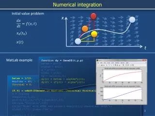
Chapter Seven. Two-Dimensional Isoparametric Elements and Numerical Integration. THE FOUR-NODE QUADRILATERAL. Coordinates of nod i. The element displacement vector. The local nodes are numbered as 1,2,3,4 in a counterclockwise fashion. SHAPE FUNCTIONS.

E N D
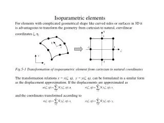
Chapter Seven Two-Dimensional Isoparametric Elements and Numerical Integration
THE FOUR-NODE QUADRILATERAL Coordinates of nod i The element displacement vector The local nodes are numbered as 1,2,3,4 in a counterclockwise fashion
SHAPE FUNCTIONS In ξ,η coordinates (natural coordinates) at nod i. i=1,2,3,4 = 0 at other nodes at nod 1 C=1/4
Displacement field within the element In the isoparametric formulation , we use the same function N to express the coordinates of a point within the element in terms of nodal coordinates
B MATRIX (I)
Another Method : iii By considering f=u in (II) we have : iv
Equation (iii) and (iv) yield : ** Equation * yield
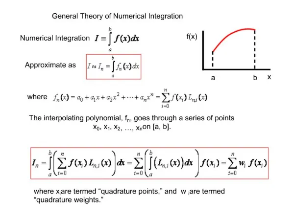
Gaussian quadrature : Consider the n-point approximation weights Gauss points n : Number of gauss points m : degree of Polynomial
One point formula : If then
Approximate Area=2f(0) Exact area = -1 0 1
Two- point formula Error =0 if
Example 7.1 evaluate for n=1 , we have for n=2 , we have for n=3 , we have
Two dimensional integrals The extension of gaussian quadrature to two –dimensional integrals
Stiffness integration Let φ represent the ijth element in the integrand If we use a 2×2 rule then:
Stress calculations Example 7.1 Consider a rectangular element as shown in fig .assume plane stress condition , E= 30×10^6 psi ,v=0.3, and Evaluate J,B and σ at ξ=0,η=0
SOLUTION From Eqs. ** Evaluating G in Eq. *** at ζ=η=0 and using B=AG
Comment on degenerate quadrilaterals In some situations, quadrilaterals elements degenerate into triangles. Numerical integration will permit the use of such elements But the errors are higher than regular elements.
Quadrilateral Higher-order elements For 4-node quadrilateral element For 9-node quadrilateral element
9-node quadrilateral element For example at nod 1:
16-node quadrilateral element(4th order) 7 (1/3,-1/3)
Triangular Higher-order elements For 3-node triangle element For 6-node triangle element
Midside node The midside node should be as near as possible to the center of the side The node should not be outside of ¼< s/l <3/4 . l