Download
1 / 47
470 likes | 603 Views
CSE 332 Data Abstractions: Introduction to Parallelism and Concurrency. Kate Deibel Summer 2012. Where We Are. Last time, we introduced fork-join parallelism Separate programming threads running at the same time due to presence of multiple cores Threads can fork off into other threads

E N D
CSE 332 Data Abstractions:Introduction to Parallelism and Concurrency Kate Deibel Summer 2012 CSE 332 Data Abstractions, Summer 2012
Where We Are Last time, we introduced fork-join parallelism • Separate programming threads running at the same time due to presence of multiple cores • Threads can fork off into other threads • Said threads share memory • Threads join back together We then discussed two ways of implementing such parallelism in Java: • The Java Thread Library • The ForkJoin Framework CSE 332 Data Abstractions, Summer 2012
Ah yes… the comfort of mathematics… Enough Implementation:Analyzing Parallel Code CSE 332 Data Abstractions, Summer 2012
Key Concepts: Work and Span Analyzing parallel algorithms requires considering the full range of processors available • We parameterize this by letting TP be the running time if P processors are available • We then calculate two extremes: work and span Work: T1How long using only 1 processor • Just "sequentialize" the recursive forking Span: T∞ How long using infinity processors • The longest dependence-chain • Example: O(logn) for summing an array • Notice that having > n/2 processors is no additional help (a processor adds 2 items, so only n/2 needed) • Also called "critical path length" or "computational depth" CSE 332 Data Abstractions, Summer 2012
The DAG A program execution using fork and join can be seen as a DAG • Nodes: Pieces of work • Edges: Source must finish before destination starts A fork "ends a node" and makestwo outgoing edges • New thread • Continuation of current thread A join "ends a node" and makes a node with two incoming edges • Node just ended • Last node of thread joined on CSE 332 Data Abstractions, Summer 2012
Our Simple Examples fork and join are very flexible, but divide-and-conquer use them in a very basic way: • A tree on top of an upside-down tree divide base cases conquer CSE 332 Data Abstractions, Summer 2012
What Else Looks Like This? Summing an array went from O(n) sequential to O(logn) parallel (assuming a lot of processors and very large n) Anything that can use results from two halves and merge them in O(1) time has the same properties and exponential speed-up (in theory) + + + + + + + + + + + + + + + CSE 332 Data Abstractions, Summer 2012
Examples • Maximum or minimum element • Is there an element satisfying some property (e.g., is there a 17)? • Left-most element satisfying some property (e.g., first 17) • What should the recursive tasks return? • How should we merge the results? • Corners of a rectangle containing all points (a "bounding box") • Counts (e.g., # of strings that start with a vowel) • This is just summing with a different base case CSE 332 Data Abstractions, Summer 2012
More Interesting DAGs? Of course, the DAGs are not always so simple (and neither are the related parallel problems) Example: • Suppose combining two results might be expensive enough that we want to parallelize each one • Then each node in the inverted tree on the previous slide would itself expand into another set of nodes for that parallel computation CSE 332 Data Abstractions, Summer 2012
Reductions Such computations of this simple form are common enough to have a name: reductions (or reduces?) Produce single answer from collection via an associative operator • Examples: max, count, leftmost, rightmost, sum, … • Non-example: median Recursive results don’t have to be single numbers or stringsand can be arrays or objects with fields • Example: Histogram of test results But some things are inherently sequential • How we process arr[i] may depend entirely on the result of processing arr[i-1] CSE 332 Data Abstractions, Summer 2012
Maps and Data Parallelism A map operates on each element of a collection independently to create a new collection of the same size • No combining results • For arrays, this is so trivial some hardware has direct support (often in graphics cards) Canonical example: Vector addition int[] vector_add(int[] arr1,int[] arr2){ assert (arr1.length == arr2.length); result = newint[arr1.length]; FORALL(i=0; i < arr1.length; i++) { result[i] = arr1[i] + arr2[i]; } return result; } CSE 332 Data Abstractions, Summer 2012
Maps in ForkJoin Framework classVecAddextendsRecursiveAction { intlo; inthi; int[] res; int[] arr1; int[] arr2; VecAdd(intl,inth,int[] r,int[] a1,int[] a2){ … } protected void compute(){ if(hi – lo < SEQUENTIAL_CUTOFF) { for(inti=lo; i < hi; i++) res[i] = arr1[i] + arr2[i]; } else { intmid = (hi+lo)/2; VecAddleft = newVecAdd(lo,mid,res,arr1,arr2); VecAddright= newVecAdd(mid,hi,res,arr1,arr2); left.fork(); right.compute(); left.join(); } } } static final ForkJoinPoolfjPool= new ForkJoinPool(); int[] add(int[] arr1, int[] arr2){ assert (arr1.length == arr2.length); int[] ans = newint[arr1.length]; fjPool.invoke(newVecAdd(0,arr.length,ans,arr1,arr2); returnans; } CSE 332 Data Abstractions, Summer 2012
Maps and Reductions Maps and reductions are the "workhorses" of parallel programming • By far the two most important and common patterns • We will discuss two more advanced patterns later We often use maps and reductions to describe parallel algorithms • We will aim to learn to recognize when an algorithm can be written in terms of maps and reductions • Programming them then becomes "trivial" with a little practice (like how for-loops are second-natureto you) CSE 332 Data Abstractions, Summer 2012
Digression: MapReduce on Clusters You may have heard of Google’s "map/reduce" • Or the open-source version Hadoop Perform maps/reduces on data using many machines • The system takes care of distributing the data and managing fault tolerance • You just write code to map one element and reduce elements to a combined result Separates how to do recursive divide-and-conquer from what computation to perform • Old idea in higher-order functional programming transferred to large-scale distributed computing • Complementary approach to database declarative queries CSE 332 Data Abstractions, Summer 2012
Maps and Reductions on Trees Work just fine on balanced trees • Divide-and-conquer each child • Example: Finding the minimum element in an unsorted but balanced binary tree takes O(logn) time given enough processors How to do you implement the sequential cut-off? • Each node stores number-of-descendants (easy to maintain) • Or approximate it (e.g., AVL tree height) Parallelism also correct for unbalanced trees but you obviously do not get much speed-up CSE 332 Data Abstractions, Summer 2012
b c d e f front back Linked Lists Can you parallelize maps or reduces over linked lists? • Example: Increment all elements of a linked list • Example: Sum all elements of a linked list Nope. Once again, data structures matter! For parallelism, balanced trees generally better than lists so that we can get to all the data exponentially faster O(logn) vs. O(n) • Trees have the same flexibility as lists compared to arrays (i.e., no shifting for insert or remove) CSE 332 Data Abstractions, Summer 2012
Analyzing algorithms Like all algorithms, parallel algorithms should be: • Correct • Efficient For our algorithms so far, their correctness is "obvious" so we’ll focus on efficiency • Want asymptotic bounds • Want to analyze the algorithm without regard to a specific number of processors • The key "magic" of the ForkJoin Framework is getting expected run-time performance asymptotically optimal for the available number of processors • Ergo we analyze algorithms assuming this guarantee CSE 332 Data Abstractions, Summer 2012
Connecting to Performance Recall: TP = run time if P processors are available We can also think of this in terms of the program's DAG Work = T1 = sum of run-time of all nodes in the DAG • Note: costs are on the nodes not the edges • That lonely processor does everything • Any topological sort is a legal execution • O(n) for simple maps and reductions Span = T∞ = run-time of most-expensive path in DAG • Note: costs are on the nodes not the edges • Our infinite army can do everything that is ready to be done but still has to wait for earlier results • O(logn) for simple maps and reductions CSE 332 Data Abstractions, Summer 2012
Some More Terms Speed-up on P processors: T1 / TP Perfectlinear speed-up: If speed-up is P as we vary P • Means we get full benefit for each additional processor: as in doubling P halves running time • Usually our goal • Hard to get (sometimes impossible) in practice Parallelism is the maximum possible speed-up: T1/T∞ • At some point, adding processors won’t help • What that point is depends on the span Parallel algorithms is about decreasing span without increasing work too much CSE 332 Data Abstractions, Summer 2012
Optimal TP: Thanks ForkJoin library So we know T1 and T∞ but we want TP (e.g., P=4) Ignoring memory-hierarchy issues (caching), TP cannot • Less than T1/ P why not? • Less than T∞ why not? So an asymptotically optimal execution would be: TP = O((T1 / P) + T∞) First term dominates for small P, second for large P The ForkJoin Framework gives an expected-time guarantee of asymptotically optimal! • Expected time because it flips coins when scheduling • How? For an advanced course (few need to know) • Guarantee requires a few assumptions about your code… CSE 332 Data Abstractions, Summer 2012
Division of Responsibility Our job as ForkJoin Framework users: • Pick a good parallel algorithm and implement it • Its execution creates a DAG of things to do • Make all the nodes small(ish) and approximately equal amount of work The framework-writer’s job: • Assign work to available processors to avoid idling • Keep constant factors low • Give the expected-time optimal guarantee assuming framework-user did his/her job TP =O((T1 / P) + T∞) CSE 332 Data Abstractions, Summer 2012
Examples: TP = O((T1 / P) + T∞) Algorithms seen so far (e.g., sum an array): If T1 = O(n) and T∞= O(logn) TP = O(n/P + logn) Suppose instead: If T1 = O(n2) and T∞= O(n) TP = O(n2/P + n) Of course, these expectations ignore any overhead or memory issues CSE 332 Data Abstractions, Summer 2012
Things are going so smoothly… Parallelism is awesome… Hello stranger, what's your name? Murphy? Oh @!♪%★$☹*!!! Amdahl’s Law CSE 332 Data Abstractions, Summer 2012
Amdahl’s Law (mostly bad news) In practice, much of our programming typically has parts that parallelize well • Maps/reductions over arrays and trees And also parts that don’t parallelize at all • Reading a linked list • Getting/loading input • Doing computations based on previous step To understand the implications, consider this: "Nine women cannot make a baby in one month" CSE 332 Data Abstractions, Summer 2012
Amdahl’s Law (mostly bad news) Let work (time to run on 1 processor) be 1 unit time If S is the portion of execution that cannot be parallelized, then we can define T1 as: T1= S + (1-S) = 1 If we get perfect linear speedup on the parallel portion, then we can define TP as: TP= S + (1-S)/P Thus, the overall speedup with P processors is (Amdahl’s Law): T1 / TP= 1 / (S + (1-S)/P) And the parallelism (infinite processors) is: T1 / T∞= 1 / S CSE 332 Data Abstractions, Summer 2012
Why this is such bad news Amdahl’s Law: T1 / TP= 1 / (S + (1-S)/P) T1 / T∞= 1 / S Suppose 33% of a program is sequential • Then a billion processors won’t give a speedup over 3 Suppose you miss the good old days (1980-2005) where 12 years or so was long enough to get 100x speedup • Now suppose in 12 years, clock speed is the same but you get 256 processors instead of just 1 • For the 256 cores to gain ≥100x speedup, we need 100 1 / (S + (1-S)/256) Which means S .0061 or 99.4% of the algorithm must be perfectly parallelizable!! CSE 332 Data Abstractions, Summer 2012
A Plot You Have To See Speedup for 1, 4, 16, 64, and 256 Processors T1 / TP = 1 / (S + (1-S)/P) CSE 332 Data Abstractions, Summer 2012
A Plot You Have To See (Zoomed In) Speedup for 1, 4, 16, 64, and 256 Processors T1 / TP = 1 / (S + (1-S)/P) CSE 332 Data Abstractions, Summer 2012
All is not lost Amdahl’s Law is a bummer! • Doesn’t mean additional processors are worthless!! We can always search for new parallel algorithms • We will see that some tasks may seem inherently sequential but can be parallelized We can also change the problems we’re trying to solve or pursue new problems • Example: Video games/CGI use parallelism • But not for rendering 10-year-old graphics faster • They are rendering more beautiful(?) monsters CSE 332 Data Abstractions, Summer 2012
A Final Word on Moore and Amdahl Although we call both of their work laws, they are very different entities • Moore’s "Law" is an observation about the progress of the semiconductor industry: • Transistor density doubles every ≈18 months • Amdahl’s Law is a mathematical theorem • Diminishing returns of adding more processors • Very different but incredibly important in the design of computer systems CSE 332 Data Abstractions, Summer 2012
If we were really clever, we wouldn't constantly say parallel because after all we are discussing parallelism so it should be rather obvious but this comment is getting too long and stopped being clever ages ago… Being Clever: Parallel Prefix CSE 332 Data Abstractions, Summer 2012
Moving Forward Done: • "Simple" parallelism for counting, summing, finding • Analysis of running time and implications of Amdahl’s Law Coming up: • Clever ways to parallelize more than is intuitively possible • Parallel prefix: • A "key trick" typically underlying surprising parallelization • Enables other things like packs • Parallel sorting:mergesort and quicksort (not in-place) • Easy to get a little parallelism • With cleverness can get a lot of parallelism CSE 332 Data Abstractions, Summer 2012
The Prefix-Sum Problem Given int[]input, produce int[]outputsuch that: output[i]=input[0]+input[1]+…+input[i] A sequential solution is a typical CS1 exam problem: int[] prefix_sum(int[] input){ int[] output = newint[input.length]; output[0] = input[0]; for(inti=1; i < input.length; i++) output[i] = output[i-1]+input[i]; return output; } CSE 332 Data Abstractions, Summer 2012
The Prefix-Sum Problem Above algorithm does not seem to be parallelizable: • Work: O(n) • Span: O(n) It isn't. The above algorithm is sequential. But a different algorithm gives a span of O(logn) int[] prefix_sum(int[] input){ int[] output = newint[input.length]; output[0] = input[0]; for(inti=1; i < input.length; i++) output[i] = output[i-1]+input[i]; return output; } CSE 332 Data Abstractions, Summer 2012
Parallel Prefix-Sum The parallel-prefix algorithm does two passes • Each pass has O(n) work and O(logn) span • In total there is O(n) work and O(logn) span • Just like array summing, parallelism is n / logn • An exponential speedup The first pass builds a tree bottom-up The second pass traverses the tree top-down Historical note: Original algorithm due to R. Ladner and M. Fischer at the UW in 1977 CSE 332 Data Abstractions, Summer 2012
Parallel Prefix: The Up Pass We build want to a binary tree where • Root has sum of the range [x,y) • If a node has sum of [lo,hi) and hi>lo, • Left child has sum of [lo,middle) • Right child has sum of [middle,hi) • A leaf has sum of [i,i+1), which is simply input[i] It is critical that we actually create the tree as we will need it for the down pass • We do not need an actual linked structure • We could use an array as we did with heaps CSE 332 Data Abstractions, Summer 2012
Parallel Prefix: The Up Pass This is an easy fork-join computation: buildRange(arr,lo,hi) • If lo+1 == hi, create new node with sum arr[lo] • Else, create two new threads:buildRange(arr,lo,mid) and buildRange(arr,mid+1,high)where mid = (low+high)/2and when threads complete, make new node with sum = left.sum + right.sum Performance Analysis: • Work: O(n) • Span: O(log n) CSE 332 Data Abstractions, Summer 2012
Up Pass Example range 0,8 sum fromleft 76 range 0,4 sum fromleft range 4,8 sum fromleft 40 36 range 0,2 sum fromleft range 2,4 sum fromleft range 4,6 sum fromleft range 6,8 sum fromleft 10 26 30 10 r 0,1 s f r 1,2 s f r 2,3 s f r 3,4 s f r 4,5 s f r 5,6 s f r 6,7 s f r 7.8 s f 6 4 16 10 16 14 2 8 input 6 4 16 10 16 14 2 8 output CSE 332 Data Abstractions, Summer 2012
Parallel Prefix: The Down Pass We now use the tree to get the prefix sums using an easy fork-join computation: Starting at the root: • Root is given a fromLeft of 0 • Each node takes its fromLeft value and • Passes to the left child: fromLeft • Passes to the right child: fromLeft + left.sum • At leaf for position i, output[i]=fromLeft+input[i] Invariant: fromLeftis sum of elements left of the node’s range CSE 332 Data Abstractions, Summer 2012
Parallel Prefix: The Down Pass Note that this parallel algorithm does not return any values • Leaves assign to outputarray • This is a map, not a reduction Performance Analysis: • Work: O(n) • Span: O(log n) CSE 332 Data Abstractions, Summer 2012
Down Pass Example range 0,8 sum fromleft 76 0 range 0,4 sum fromleft range 4,8 sum fromleft 40 36 0 36 range 0,2 sum fromleft range 2,4 sum fromleft range 4,6 sum fromleft range 6,8 sum fromleft 10 26 30 10 0 10 36 66 r 0,1 s f r 1,2 s f r 2,3 s f r 3,4 s f r 4,5 s f r 5,6 s f r 6,7 s f r 7.8 s f 6 4 16 10 16 14 2 8 6 26 36 52 66 0 10 68 input 6 4 16 10 16 14 2 8 output 6 10 26 36 52 66 68 76 CSE 332 Data Abstractions, Summer 2012
Sequential Cut-Off Adding a sequential cut-off is easy as always: • Up Pass: Have leaf node hold the sum of a range instead of just one array value • Down Pass:output[lo] = fromLeft + input[lo]; for(i=lo+1; i < hi; i++) output[i] = output[i-1] + input[i] CSE 332 Data Abstractions, Summer 2012
Generalizing Parallel Prefix Just as sum-array was the simplest example of a common pattern, prefix-sum illustrates a pattern that can be used in many problems • Minimum, maximum of all elements to the left of i • Is there an element to the left of i satisfying some property? • Count of elements to the left of i satisfying some property That last one is perfect for an efficient parallel pack that builds on top of the “parallel prefix trick” CSE 332 Data Abstractions, Summer 2012
Pack (Think Filtering) Given an array input and boolean function f(e)produce an array output containing only elements e such that f(e) is true Example: input [17, 4, 6, 8, 11, 5, 13, 19, 0, 24] f(e): is e > 10? output [17, 11, 13, 19, 24] Is this parallelizable? Of course! • Finding elements for the output is easy • But getting them in the right place seems hard CSE 332 Data Abstractions, Summer 2012
Parallel Map + Parallel Prefix + Parallel Map • Use a parallel map to compute a bit-vector for true elements input [17, 4, 6, 8, 11, 5, 13, 19, 0, 24] bits [ 1, 0, 0, 0, 1, 0, 1, 1, 0, 1] • Parallel-prefix sum on the bit-vector bitsum [ 1, 1, 1, 1, 2, 2, 3, 4, 4, 5] • Parallel map to produce the output output [17, 11, 13, 19, 24] output =new array of size bitsum[n-1] FORALL(i=0; i < input.length; i++){ if(bits[i]==1) output[bitsum[i]-1] = input[i]; } CSE 332 Data Abstractions, Summer 2012
Pack Comments First two steps can be combined into one pass • Will require changing base case for the prefix sum • No effect on asymptotic complexity Can also combine third step into the down pass of the prefix sum • Again no effect on asymptotic complexity Analysis: O(n) work, O(logn) span • Multiple passes, but this is a constant Parallelized packs will help us parallelize sorting CSE 332 Data Abstractions, Summer 2012
Welcome to the Parallel World We will continue to explore this topic and its implications In fact, the next class will consist of 16 lectures presented simultaneously • I promise there are no concurrency issues with your brain • It is up to you to parallelize your brain before then The interpreters and captioner should attempt to grow more limbs as well CSE 332 Data Abstractions, Summer 2012