Download
1 / 53
530 likes | 592 Views
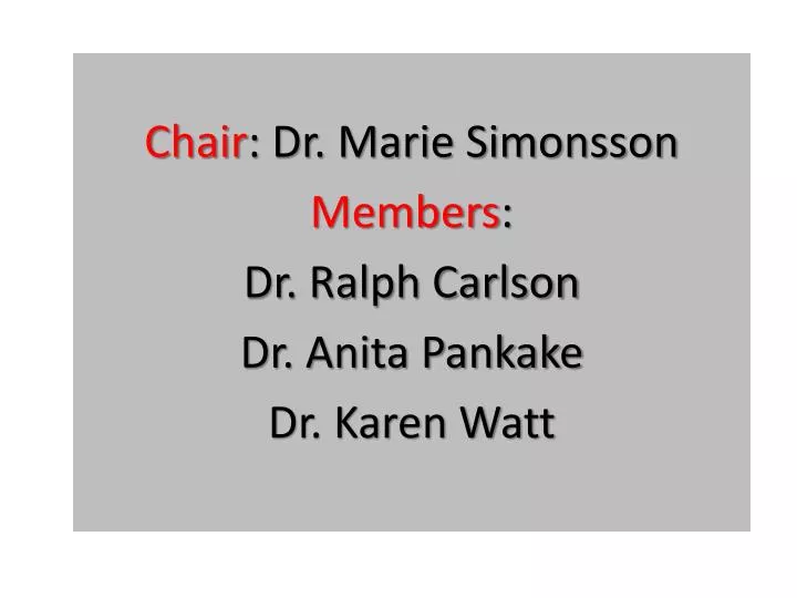
Chair : Dr. Marie Simonsson Members : Dr. Ralph Carlson Dr. Anita Pankake Dr. Karen Watt. AN INVESTIGATION OF HIGH SCHOOL DUAL ENROLLMENT PARTICIPATION AND ALLIED HEALTH PROGRAM ENROLLMENT IN A SOUTH TEXAS UNIVERSITY. Dissertation Defense by Marti Flores Fall 2010 *Define DE Programs

E N D
Chair: Dr. Marie Simonsson Members: Dr. Ralph Carlson Dr. Anita Pankake Dr. Karen Watt
AN INVESTIGATION OF HIGH SCHOOL DUAL ENROLLMENT PARTICIPATION AND ALLIED HEALTH PROGRAM ENROLLMENT IN A SOUTH TEXAS UNIVERSITY Dissertation Defense by Marti Flores Fall 2010 *Define DE Programs and AH Programs (Exclusive/5 AH )
National Shortage of Healthcare Professionals Population Growth Survival Rates BB Retiring Prediction Overall Transition HS Students into Higher Education: Particularly AH Professions Dual Enrollment
Introduction Demand HC (BB=Silver) & (Surv. Rates=Interventions) (Lang, 2009) Seamless Transition HS – PS Education Gap (Conley et al., 2006) Postsecondary enrollments 5.3 million healthcare workers (PRWEB, 2007) Support System -Dual enrollment (Andrews, 2004)
Need of the Study • Hughes, Karp, Fermin, & Bailey, 2005 = Nat’al Study Pathways-Persistence? • Olson, 2006 = Scarce data – Accel program effectiveness • Smith, 2007 = At-risk, low income, and minority students • Swanson, 2008 = Limited evidence persistence - graduation • Lee, 2009 = Lack of studies concerning factors = AA Purpose of the Study • Existing Literature/Value DE • Investigate factors motivated (student report) • Factors contributing to success • Proportion of total variance in AA attributed to 5 IVs
Review of the Literature Supporting Views Review of the Literature Opposing Views
Research Questions (Prior to Data Reduction) 1.What motivated college students to enroll in health science technology (HST) dual enrollment courses while they were in high school? 2. What factors or variables do college students who enrolled in health science technology (HST) dual enrollment courses believe contribute to their academic success? 3. What proportion of the total variance in academic achievement may be attributed to academic resources, dual enrollment, parental education, persistence, and social interactions?
Research Design/Methods A QUALquan mixed method design was used for the present study (Gay, Mills, Airsian, 2006). IRB Approval from both institutions, entry access granted, consent forms Qualitative :Phenomenological Approach via FG: - Group 1 :12/15 participants (9F -3M);60 minute session - Group 2: 9/14 participants (7F – 2M);75 minute session Quantitative - ID Target Population –Survey (11Q-60 Item): MLR - 86 surveys – 38.4% return rate
Survey/CodingExample 1 What is your gender? A. Male B. Female Scaling level of the data above: Coded the data Male (0) and Female (1)
Survey/Coding Example 2 Father’s level of education: Less than high school High school or GED Some college, including vocational/technical Bachelor’s Degree Graduate (Master’s or Doctorate) I do not know Code? Coded the data: a = 1, b = 2, c = 3, d = 4, e = 5
Survey/Coding Example 3 How often do you visit with your professor outside the classroom? I do not visit Weekly Once a semester More than once a semester Code? Coded the data: a = 1 b = 4 c = 2 d = 3
Pre-Analysis:Quantitative Distribution Graph Box-Whisker’s Plot Stem –Leaf Plots Exploratory/Measurement Analysis: - Master data Spreadsheet of Raw Data: Carefully SPSS-17 (5 constructs and 22 IV variables) - Descriptive Data - √ (N); min/max; Std. Dev.; Skewness; Kurtosis Shape –Kolmogorov N Test Linearity –Outliers Shape of the Distribution
Pre-Analysis:Quantitative Distribution Graph HSRankskewness =+4.328 OutClassMskewness= -1.41 Skewness: Symmetry of the Distribution Alpha Error : And ? Variance is due to Regression Divide it by std. error
Pre-Analysis:Quantitative Box-Whisker’s Plot 3 rd Quartile Linearity –Outliers Median Exploratory/Measurement Analysis: 1st Quartile
Review your Descriptive Statistics Results Next Slide has steps for Descriptive Statistics Then Scroll through the SPSS results you obtained See next slide
Steps for Descriptive Statistics SPSS – Highlight all the variables Go to Analyze Go to Descriptive Statistics Go to Descriptives Move the variables into “variable” slot and go to “options” Click on the choices (Mean, Std. Dev., Variance, etc) Results on the next slide
Results of Descriptive Statistics Note: N for each column [excellent checkpoint] Note: Mean and Median Note Skewness [close to 0][Type I alpha error][+skewness mean is higher than median] [- skewness mean is lower than the median] Note Variance [Don’t want 0] Note: Kurtosis [- platy & + lepto]
Steps for Explore SPSS – Highlight all the variables Go to Analyze Go to Descriptive Statistics Go to Explore Move ALL the variables into the dependent variable Click on Statistic Description 95% CI Click on Continue and go to Plots Click O’K to run the data Select stem/leaf; histogram, normal plot
Results of Explore (Normality Test) Tests of Normality Kolmogorov-Smirnova Statistic df Sig. AcadAch.074 86 .200* a. Lilliefors Significance Correction *. This is a lower bound of the true significance.
Psychometric Properties - Psychometric Properties of the IV: Item Analysis and Discriminatory Index : Socialization construct: inter-item correlation to make sure they were measuring the same phenomenon. One of the four socialization items was contributing to noise and lowering our Cronbach’s alpha reliability value (consistency). It was removed and the Cronbach alpha reliability level changed from .512 to .594
Steps to Reliability First acquire reliability Cronbach’s alpha on 4 socialization variables Click on analyze Click on Scale Click on Reliability Move in (4) socialization variables For Model Click on Alpha
Cronbach’s Alpha Reliability of 4 Socializ. Variables Reliability Statistics Cronbach's Alpha N of Items .512 4
Step for Discrim. Index Now aggregate the 4 items under socialization into one composite or total score Go to Transform Compute variable Under target variable enter new name: “NewTotalSoc” Enter the (4) socialization variables and click O’K (XXX+XXX+XXX+XXX) Under the variable view, you should see the new variable name (NewTotalSocialization) Then go to Analyze*Correlate*Bivariate*enter the Newtotalsocial variable PLUS the other (4) social variables (how do the four items correlate with the total score?) Click the Pearson ( r) correlation coefficient and 2 tailed test Click O’K ---- See next slide
Review your Psychometric Testing Results: Reliability Using the (4) socialization items and the new aggregate total score
Inter- Item Correlation newtotalsoc OutAct OutClassMa OutProf OutCounselor newtotalsocPearson Correlation 1 .798** .563** .783**.300** Sig. (2-tailed) .000 .000 .000 .005 N 86 86 86 86 86 OutAct Pearson Correlation .798** 1 .286** .514** .055 Sig. (2-tailed) .000 .007 .000 .615 N 86 86 86 86 86 OutClassMaPearson Correlation .563** .286** 1 .169 -.161 Sig. (2-tailed) .000 .007 .120 .137 N 86 86 86 86 86 OutProfess Pearson Correlation .783** .514** .169 1 .194 Sig. (2-tailed) .000 .000 .120 .074 N 86 86 86 86 86 OutCounselor Pearson Correlation .300** .055 -.161 .194 1 Sig. (2-tailed) .005 .615 .137 .074 N 86 86 86 86 86 **. Correlation is significant at the 0.01 level (2-tailed). Discriminatory Index
Review your Psychometric Testing Results: Reliability Now take the three significant socialization items and run the reliability test – see next slide
Reliability Statistics Cronbach's Alpha N of Items .512 4 Cronbach’s Alpha Reliability of 3 Socializ. Variables Without Socialization with Counselor: Almost 60% of the variance is true or reliable Reliability Statistics Cronbach's Alpha N of Items .594 3
Data Analysis Intercorrelation Matrix Bivariate Correlational Analysis Pearson (r ) Corr. Coef : High Correlation with the DV and little or no correlation among the other IV 11 of the 22 variables had a significant correlation with the DV (86 surveys X 60 items)
Steps for Bivariate Correlation Go to Analyze Correlate Bivariate Move in all variables (DV and IV) Select Pearson (r ) correlation coefficient Select 2 tailed test Click O’K to run the data
Review your Correlation Results Correlation Coefficient
Remember 11 of the 22 variables had a significant correlation with the DV (86 surveys X 60 items)
Data Reduction Factor Analysis – a statistical method used to describe variability among observed variables Helped with data reduction - variables testing the same underlying phenomenon
Steps for Factor Analysis Click on Analyze Dimension Reduction Factor Input 11 IVs and then go to Rotation Select Varimax Click O’K
Review your Factor Analysis Results Data Reduction
Results of Factor Analysis Scree Plot Principle Component Analysis Eigenvalue > 1 no multicollinearity 68.9% of the variance explained Varimax Rotation: Simple Structure Justification?
Summary Research questions drive the methodology Data Entry Vital Descriptive Statistics Cronbach’s Alpha Reliability Discriminatory Index Importance of Factor Analysis Next Class : Multiple Regression Analysis
Class Meeting #2 Review previous material Descriptive Statistics Cronbach’s Alpha Reliability Discriminatory Index Importance of Factor Analysis Today: Multiple Regression Analysis
Regression Analyses Factor 1 Label: X1 HS Achievement (HSAch) as measured by TAKS Factor 2 Label: X2 HS Performance (HSPerf) as measured by -HS GPA - HSRank - Num DE Credits Factor 3 Label: X3Aptitude (Apt) as measured by SAT Factor 4 Label: X4 proActive as measured by Persistence Yr1 and OutProf DV (Y) Academic Achievement as measured by college GPA (continuous data interval scaling level) Null Hypothesis: H0 Academic Achievement (Y) is not a function of High School Achievement, High School Performance, Aptitude, and ProActive. REJECTED
Regression: Full Model • 37% of the variance in academic achievement was accounted for or explained by the four IV. • Findings were significant at alpha .01 level • Critical F was 3.65 and the derived F was 11.92; therefore, the H0 was Model Summary Model R (β) R Square (β2) Adjusted R Square Std. Error of the Estimate 1 .609a .371 .340 .58580 a. Predictors: (Constant), ALL (4)proActive, Apt,HSAch, HSperformance p = .05 REJECTED • Academic achievement (Y) IS a function of high school achievement, high school performance, aptitude, and proActive.
Regression: All Possible Procedures (Backward Elimination Procedure) Unique V Independent Independent β2β2Unique Variables Variable Removed Full Variance Model X1,X2, X3 X4(proAct) .37 .34 .03 X1, X2, X4 X3 (Aptitude) .37 .36 .01 X1, X3, X4 X2(HSPerf) .37 .29 .08 X2, X3, X4 X1 (HSAch) .37 .33 .04 X2 HS Performance (HSPerf) as measured by -HS GPA - HSRank - Num DE Credits X1 HS Achievement (HSAch) as measured by TAKS
Regression: All Possible Procedures Independent Independent β2β2Unique Variables Variables Removed Full Variance X3, X4 X1, X2.37 .20 .17 X2, X4 X1, X3 .37 .31 .06 X2, X3 X1, X4 .37 .30 .07 X1, X4 X2, X3 .37 .27 .10 X1, X3 X2, X4 .37 .24 .13 X1, X2 X3, X4 .37 .33 .04 X2 HS Performance (HSPerf) as measured by -HS GPA - HSRank - Num DE Credits X1 HS Achievement (HSAch) as measured by TAKS “Best Fit”
Regression: All Possible Procedures “Best Fit” Independent Independent β2β2Unique Variables Variables Removed Full Variance X1 X2, X3, X4 .37 .21 .16 X2X1, X3, X4 .37 .27 .10 X3 X1, X2, X4 .37 .12 .25 X4 X1, X2, X3 .37 .12 .25 X2 HS Performance (HSPerf) as measured by -HS GPA - HSRank - Num DE Credits X1 HS Achievement (HSAch) as measured by TAKS
Discussion of Findings What Does This All Mean? Quantitative: - 37% of the total variance in AA is attributed to 4 IVs X2 HS Performance (HSPerf) as measured by -HS GPA - HSRank - Num DE Credits X1 HS Achievement (HSAch) as measured by TAKS “Best Fit”
Assumptions of the Study Qualitative Research - Truthfulness of the FG participants - UTB Data accurate/factual - Check and Recheck FG responses Quantitative Research - Normality of the data - Linearity - Homoscedasticity(conditional distributions)
Limitations of the Study Other academic groups - Transferability - Generalization Gender prominence Choice of educational institution Recollections Existential nature of the quantitative data “moment in time”
Implications Implications for Theory – Support Dr. Vincent Tinto’s model of student departure: Academic variables are valuable – “What student brings from HS” *X1 HS Achievement (HSAch) as measured by TAKS *X2 HS Performance (HSPerf) as measured by -HS GPA - HSRank - Num DE Credits Dr. Vincent Tinto’s Post Matriculation Theory with social interactions – “persistence and socialization with prof.” X4 proActive as measured by Persistence Yr1 and OutProf Implications for Practice – Preparatory programs’ academic and financial oversight Retention strategies – AH- Motivation factors/obstacles Implementation HS Advisement Programs –”Grades” Need for College Rigor –Mixed Classes – Affiliation, Mtgs, Prof. Dev.