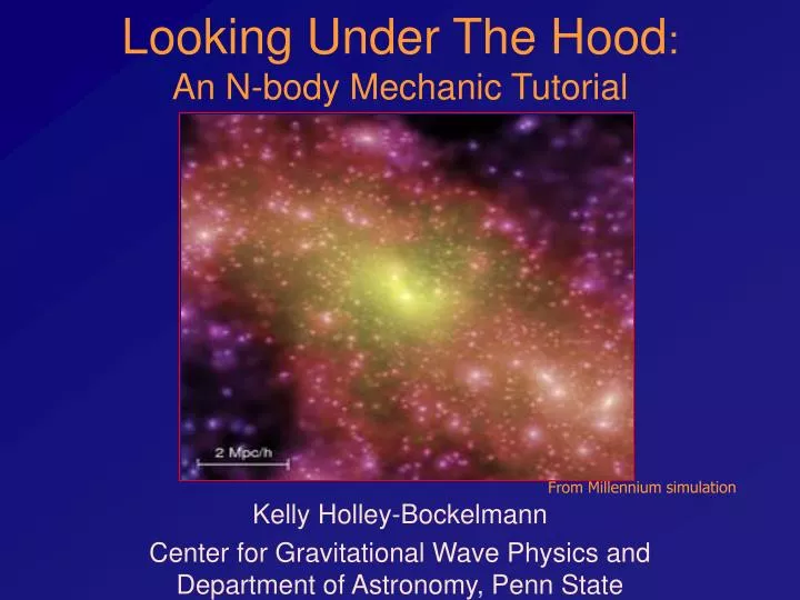
Looking Under The Hood : An N-body Mechanic Tutorial

Looking Under The Hood: An N-body Mechanic Tutorial Kelly Holley-Bockelmann Center for Gravitational Wave Physics and Department of Astronomy, Penn State From Millennium simulation

N-body simulations can track structures as they assemble within a cosmological volume Matthias Steinmetz matter = 0.35 +/- 0.1baryon= 0.045 +/- 0.15dark energy = 0.65 +/- 0.1

Or how galaxies harrass one another at late times within a galaxy cluster

How an individual galaxy responds to perturbations And how well the dark matter couples to the galaxy’s evolution

They can also provide a window into the arrangement of the dark matter within a halo 5123 particles in 4803 Mpc –then zoom in and repopulate Volker Springel

We’ll concentrate on equilibrium galaxies …which totally neglects a large set of n-body simulations • cosmological simulations • gas • solar system/ few body • direct n-body simulations • black holes with ‘realistic’ gravity • non-equilibrium experiments --like mergers or collapse • If you’re interested in this stuff, we can do another tutorial later

Collisionless Stellar Systems 1 Tc ~ Crossing time Gh Tc << Tr N Tr ~ Tc Relaxation time (NOT ‘collision time’) 8 ln N Tc=106 years Tr=109 years N ~ 106 stars Tc=108 years Tr>1010 years N ~ 1011 stars

The Collisionless Boltzmann Equation Let the total mass in stars within the phase space volume d3r d3v at time t be: f(r,v,t) d3r d3v Distribution function  f  f  f - + V • = 0 Completely describes the evolution of the system. Then: •  v  t  r  2 = 4G f d3v But..impractical to solve in 3-d via finite difference methods Where:

dri dvi = vi = - r=ri dt dt Another approach: N-body realization Build model at some initial time t0 with N particles such that the probability of a particle at r,v is proportional to f(r,v,t0) Evolve this N-body realization according to very simple equations of motion: Problem: Assume 109 particles distributed with 1 kpc resolution in a 1 Mpc cube. If we want to evolve a system for 100 timesteps, that’s 1020 calculations! If each one is ~ 10 Floating Point Operations, that’s 1021 FLOPs. At supercomputer speed of 1013 operations/second, that’s a 3 year calculation…sucks to be me.

N-body simulations are limited by: • numerical errors • round-off error • ‘truncation’ error in timestep • dynamic range effects • discreteness • bugs • sub-grid physics • oversimplification of the model

Early N-body Mechanic To consider simultaneously all these causes of motion and to define these motions by exact laws allowing of convenient calculation exceeds, unless I am mistaken, the forces of the entire human intellect. --Newton

Collisions of “light bulb” galaxies • Force of Gravity  1/r2, as does light intensity • Holmberg built special purpose computer using 74 light bulbs (37 for each of two colliding galaxies) • They were on ruled graph paper, each was unscrewed in turn and replaced with a 4-sided photometer to measure the force. Positions and velocities were updated • Digital computers didn’t integrate 74 particles for 25 years!

Modern N-body Simulations Describe initial conditions as a distribution of massive particles Calculate forces between them efficiently follow their motions in time

First Step: Build a Galaxy Most studies need a model in dynamical equilibrium – Defined by a potential-density pair such that the distribution function is time-independent. Let’s go through the exercise of making a very simple galaxy model, the Plummer sphere (polytrope of index 5)

1 (r) = - G M ( r2 + a2)1/2 Building an Equilibrium Plummer Sphere Assume spherical symmetry, so that (r)=(r ), (r )=(r ), and that the velocity distribution is isotropic. In general, spherical symmetry in position space can still allow a cylindrical symmetry in velocity space – i.e. the distribution function is a function of energy *and* angular momentum. However, by assuming isotropy, we assert that: ƒ(E, J)=f(E)

3 M a2 (r) = 4 (r2 + a2)5/2  m(r ) = 4r2(r ) dr 0 Getting the density: To find the density, just solve Poisson’s equation: Now we just throw particles down randomly according to this density – how? Introducing the cumulative mass distribution: r So m(r )/M is a number between 0 and 1…looks like a good form for a random number!

Laying down the positions So, we can pick a random number between 0 and 1 to get the fractional mass, but what we really want is the *position* at that mass --- r(m) rather than m(r ) m(r ) = r3(r2+a)-3/2 r(m ) = a (rand-2/3 –1)-1/2

vesc  (r ) = f(E) 4v2dv 0 Laying down the velocities We’re going to assign random isotropic velocities so that they obey the distribution function f(r,v). So, first we gotta determine f(r,v) from (r) and (r )… Recall that f(r,v) dr dv is the mass within a volume element dr dv Recall, too that we can write f(E)=f(r,v) in a spherical isotropic system, so f(E) dr dv is the mass within a volume element dr dv Ahem, notice it’s not f(E) dE, like I bet you were tempted to say Density is essentially a 3-d projection of the 6-d phase space

  (r ) = 25/2 f() (-)1/2 d 0 1 d2 d 1 d f() = 8d2 -   d =0 Laying down the velocities (con’t) where vesc = 2 (r2 +1)-1/4 And inverting this gives you the distribution function:

dg(q) = q (2- 9q2) (1- q2)5/2  0.092 dq Laying down the velocities (con’t) 384 2 ()7/2 r2v2drdv 7m f(r,v)dr dv = Probability g(v) to have velocity v at position r  ()7/2v2 dv change variables q = v/vesc: g(q)=(1-q2)7/2 q2 Rejection technique, choose q such that it’s weighted by g(q) Choose random variables such that q  {0,1} and g(q)  {0,0.1}

Ta-da! – spherical, isotropic system in equilibrium • disks and triaxial spheriods • multicomponent systems • anisotropy • increased resolution – multimass • black holes • non-equilibrium experiments

Example: Building BH-Embedded Triaxial Models • Moderate Triaxiality (0.25 < T < 0.75) • Cuspy initial inner density profile • Variable black hole masses To resolve the BH, a multimass scheme: m(E,J)  rp where rp = (r vt)2 E+ M/a To resolve the dynamics: • N=10,000,000 • multiple timestep, 4th order Hermite integrator

N-body on the cheap Calculating pair-wise Newtonian gravitational forces by direct summation is an N2 problem – 1010 stars and 10HUGE dark matter particles Newton was a smart guy Reduce the calculation to O(N) by writing the potential as a basis expansion (r ) =  Anlmnlm ( r ) , ( r) =  Anlmnlm ( r) nlm nlm nl 2l+3 rl nlm = Cn () 4 Ylm (,) 2 2 r( 1+r)2l+3 2l+3 - rl nlm = Cn () 4 Ylm (,) 2 ( 1+r)2l+1 Anlm =  mk nlmrk,k,k* k

N-body on the cheap: Hardware version • Grape-6 – special purpose computer to directly calculate newtonian gravity between particles • 32 chips/board , 64 boards  63 Tflops! • particles are set into SRAM, then injected into a pipeline where acceleration is calculated

N-body on the cheap: Treecode version Assume that at large distances, the gravitational force of many particles in a cell can be approximated by the force from the center of mass of the cell. • Divide cube into 8 subcubes • if zero particles in subcube, delete • if subcube contains more than 1 body, recursively subdivde O(N logN) calculation

Integrators Single timestep vs. individual timesteps Symplectic  time-reversible -- built-in energy conservation Galaxy/cosmological simulations can tolerate a lot more positional, energy errors than solar system sims  potential fluctuations cause bigger errors • Leapfrog – second order (accuracy in position/energy increases by at least a factor of 100 ift cut by 10…truncation error  t2) vn+1/2 = vn + ½ t a(rn) rn+1 = rn +t vn+1/2 vn+1 = vn+1/2 + ½ t a(rn+1) n-1 n-1/2 n n+1/2 n+1 n+3/2 r, a v r, a v r, a v

N  s = G aji Mj junk rji3 j=1 ji N N  Mk  Mk rki N aji = G rkj  vji 3(rji vji) rji • rkj3 rki3 j = G Mj k=1 kj k=1 ki rji3 rji5 j=1 ji ri+1 = ½ (vi+vi+1)t +1/12 (ai – a i+1) t2 vi+1 = ½ (ai+ai+1)t +1/12 (ji – j i+1) t2 • Hermite integrator  4th order -- all about the ‘jerk’  r , the highest derivative of r that requires only 1 pass through the particles (see also snap, crackle and pop…) Integrators, con’t where vji = vj-vi where aji = aj-ai

We’ll concentrate on equilibrium galaxies …which totally neglects a large set of n-body simulations • cosmological simulations • gas • solar system/ few body • direct n-body simulations • black holes with ‘realistic’ gravity • non-equilibrium experiments --like mergers or collapse • If you’re interested in this stuff, we can do another tutorial later

Looking Under The Hood : An N-body Mechanic Tutorial