Download

1 / 28
280 likes | 291 Views
Approximation on Finite Elements. Bruce A. Finlayson Professor Emeritus of Chemical Engineering. Outline Approximation on finite elements Mesh refinement Calculus of variations Galerkin method. The function x^2 exp(y-0.5) looks like this when plotted:. Approximation on finite elements.

E N D
Approximation on Finite Elements Bruce A. Finlayson Professor Emeritus of Chemical Engineering Outline Approximation on finite elements Mesh refinement Calculus of variations Galerkin method
Approximation on finite elements • Break the region into small blocks, and color each block according to an average value in the block. • The approximation depends on the number of blocks.
Divide the domain into blocks (finite elements) and assign an average value to each block.
Write the approximation as a linear combination of trial functions, each of which takes the value one in one block and zero in all the other blocks.
Using color to represent the value, this is the solution with N x N blocks, N=4
This is mesh refinement. • Notice how the picture got better and better the more squares we took. • We approximated the function on each block - a finite element approximation. • We get a better approximation when we use small finite elements. • As the number of blocks increases, the picture approaches that of a continuous function.
Let functions in the block be bilinear functions of u and v, 0 ≤ u,v ≤ 1. • N1 = (1 - u) (1 - v) • N2 = u (1 - v) • N3 = u v • N4 = (1 - u) v • The value of each Ni is 1.0 at one corner and zero at the other three corners. • Example:N3(1,1) = 1; N3(0,1) = N3(1,0) = N3(0,0)=0
Compare constant interpolation on finite elements with bilinear interpolation on finite elements. A better approximation is achieved using fewer blocks when the trial function is a higher degree polynomial. Constant interpolation with 32x32 = 1024 blocks. Bilinear interpolation with 4x4 = 16 blocks.
Instead of matching the function at the block-corners, find the best interpolant by minimizing the mean square difference between the approximation and the exact function. Still use finite elements, but bilinear approximations. The approximation - Minimization - Equations to solve - Test function Function we’d like to be zero
What do you do if you don’t know the function? When the function is the solution to a differential equation, for example, the Calculus of Variations can be used to find the approximation, as follows.
Calculus of Variations The function that satisfies this differential equation: minimizes this integral (this must be proved for each equation): The same approach can be taken: to satisfy the differential equation, one approximates the integral on the finite element blocks and finds the minimum.
We choose finite element functions which satisfy the boundary conditions, and then find the values of the parameters that make the integral a minimum. Minimize this integral with respect to the
The solution with linear elements on 312 triangles (177 nodes) is:
The solution with linear elements on 1248 triangles (665 nodes) is:
Finite Element Variational Method • Divide the domain into small regions. • Write a low degree polynomial on each small region: constant, bilinear, biquadratic. These are the trial functions. • Write the solution as a series of trial functions. • Determine the coefficients by minimizing an integral. (The trick is to know what integral to use.)
Galerkin Finite Element Method • If a variational principle exists, the Galerkin method is the same as the variational method. It applies when there is no integral to be minimized or made stationary. • The same finite elements can be used. • The finite element approximation is put into the differential equation, and this is called the residual. It needs to be zero. • Now the residual is made orthogonal to each trial function; if this is done for infinitely many trial functions, or test functions, then the residual is zero. In practice the approximation is better the smaller the residual, and the approximation converges to the solution as the number of trial functions increases.
Conclusion - Three Basic Ideas • Write the solution in a series of functions, each of which is defined over small elements, using low-order polynomials. • Minimize some integral to solve a differential equation (or use Galerkin or the Method of Weighted Residuals, MWR). • Increase the number of basis functions in order to demonstrate convergence.