Download
1 / 41
410 likes | 548 Views
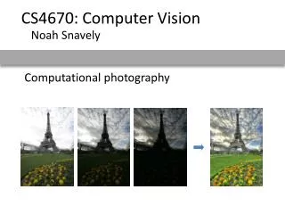
CS4670: Computer Vision. Noah Snavely. Lecture 33: Computational photography. Photometric stereo. Limitations. Big problems doesn’t work for shiny things, semi-translucent things shadows, inter-reflections Smaller problems camera and lights have to be distant calibration requirements

E N D
CS4670: Computer Vision Noah Snavely Lecture 33: Computational photography
Limitations • Big problems • doesn’t work for shiny things, semi-translucent things • shadows, inter-reflections • Smaller problems • camera and lights have to be distant • calibration requirements • measure light source directions, intensities • camera response function • Newer work addresses some of these issues • Some pointers for further reading: • Zickler, Belhumeur, and Kriegman, "Helmholtz Stereopsis: Exploiting Reciprocity for Surface Reconstruction." IJCV, Vol. 49 No. 2/3, pp 215-227. • Hertzmann & Seitz, “Example-Based Photometric Stereo: Shape Reconstruction with General, Varying BRDFs.” IEEE Trans. PAMI 2005
Finding the direction of the light source P. Nillius and J.-O. Eklundh, “Automatic estimation of the projected light source direction,” CVPR 2001
Application: Detecting composite photos Which is the real photo? Fake photo Real photo
The ultimate camera • What does it do?
The ultimate camera • Infinite resolution • Infinite zoom control • Desired object(s) are in focus • No noise • No motion blur • Infinite dynamic range (can see dark and bright things) • ...
Creating the ultimate camera • The “analog” camera has changed very little in >100 yrs • we’re unlikely to get there following this path • More promising is to combine “analog” optics with computational techniques • “Computational cameras” or “Computational photography” • This lecture will survey techniques for producing higher quality images by combining optics and computation • Common themes: • take multiple photos • modify the camera
Noise reduction • Take several images and average them • Why does this work? • Basic statistics: • variance of the mean decreases with n:
Field of view • We can artificially increase the field of view by compositing several photos together (project 2).
Improving resolution: Gigapixel images • A few other notable examples: • Obama inauguration (gigapan.org) • HDView (Microsoft Research) Max Lyons, 2003fused 196 telephoto shots
Improving resolution: super resolution • What if you don’t have a zoom lens?
Intuition (slides from Yossi Rubner & Miki Elad) For a given band-limited image, the Nyquist sampling theorem states that if a uniform sampling is fine enough (D), perfect reconstruction is possible. D D 13
2D 2D Intuition (slides from Yossi Rubner & Miki Elad) Due to our limited camera resolution, we sample using an insufficient 2D grid 14
2D 2D Intuition (slides from Yossi Rubner & Miki Elad) However, if we take a second picture, shifting the camera ‘slightly to the right’ we obtain: 15
Intuition (slides from Yossi Rubner & Miki Elad) Similarly, by shifting down we get a third image: 2D 2D 16
Intuition (slides from Yossi Rubner & Miki Elad) And finally, by shifting down and to the right we get the fourth image: 2D 2D 17
Intuition By combining all four images the desired resolution is obtained, and thus perfect reconstruction is guaranteed. 18
Example 3:1 scale-up in each axis using 9 images, with pure global translation between them 19
Dynamic Range Typical cameras have limited dynamic range
Pixel count Scene Radiance HDR images — merge multiple inputs
HDR images — merged Pixel count Radiance
Camera is not a photometer! • Limited dynamic range • 8 bits captures only 2 orders of magnitude of light intensity • We can see ~10 orders of magnitude of light intensity • Unknown, nonlinear response • pixel intensity amount of light (# photons, or “radiance”) • Solution: • Recover response curve from multiple exposures, then reconstruct the radiance map
Capture and composite several photos • Works for • field of view • resolution • signal to noise • dynamic range • Focus • But sometimes you can do better by modifying the camera…
Focus • Suppose we want to produce images where the desired object is guaranteed to be in focus? • Or suppose we want everything to be in focus?
Light field camera [Ng et al., 2005] http://www.refocusimaging.com/gallery/
Conventional vs. light field camera Conventional camera Light field camera
Light field camera • Rays are reorganized into many smaller images corresponding to subapertures of the main lens
Adaptive Optics microlens array 125μ square-sided microlenses Prototype camera • 4000 × 4000 pixels ÷ 292 × 292 lenses = 14 × 14 pixels per lens Contax medium format camera Kodak 16-megapixel sensor
What can we do with the captured rays? • Change viewpoint
All-in-focus images • Combines sharpest parts of all of the individual refocused images Using single pixel from each subimage
All-in-focus • If you only want to produce an all-focus image, there are simpler alternatives • E.g., • Wavefront coding [Dowsky 1995] • Coded aperture [Levin SIGGRAPH 2007], [Raskar SIGGRAPH 2007] • can also produce change in focus (ala Ng’s light field camera)
Why are images blurry? Camera focused at wrong distance Depth of field How can we remove the blur? Motion blur
= Motion blur • Especially difficult to remove, because the blur kernel is unknown both unknown
= = Multiple possible solutions Sharp image Blur kernel = Blurry image Slide courtesy Rob Fergus
Priors can help Priors on natural images Image A is more “natural” than image B
Natural image statistics Characteristic distribution with heavy tails Histogram of image gradients