Download
1 / 42
430 likes | 581 Views
Introduction to Cluster Analysis. Dr. Chaur-Chin Chen Department of Computer Science National Tsing Hua University Hsinchu 30013, Taiwan http://www.cs.nthu.edu.tw/~cchen. Cluster Analysis (Unsupervised Learning).

E N D
Introduction to Cluster Analysis Dr. Chaur-Chin Chen Department of Computer Science National Tsing Hua University Hsinchu 30013, Taiwan http://www.cs.nthu.edu.tw/~cchen
Cluster Analysis (Unsupervised Learning) The practice of classifying objects according to their perceived similarities is the basis for much of science. Organizing data into sensible groupings is one of the most fundamental modes of understanding and learning. Cluster Analysis is the formal study of algorithms and methods for grouping or classifying objects. An object is described either by a set of measurements or by relationships between the object and other objects. Cluster Analysis does not use the category labels that tag objects with prior identifiers. The absence of category labels distinguishes cluster analysis from discriminant analysis (Pattern Recognition).
Objective and List of References The objective of cluster analysis is to find a convenient and valid organization of the data, not to establish rules for separating future data into categories. Clustering algorithms are geared toward finding structure in the data. • B.S. Everitt, Unsolved Problems in Cluster Analysis, Biometrics, vol. 35, 169-182, 1979. • A.K. Jain and R.C. Dubes, Algorithms for Clustering Data, Prentice-Hall, New Jersey, 1988. • A.S. Pandya and R.B. Macy, Pattern Recognition with Neural Networks in C++, IEEE Press, 1995. • A.K. Jain, Data clustering : 50 years beyond K-means Pattern Recognition Letters, vol.31, no.8, 651-666, 2010.
dataFive.txt Five points for studying hierarchical clustering 2 5 2 (2I4) 4 4 8 4 15 8 24 4 24 12
Example of 5 2-d vectors 5 3 1 24
Clustering Algorithms • Hierarchical Clustering Single Linkage Complete Linkage Average Linkage Ward’s (variance) method • Partitioning Clustering Forgy K-means Isodata SOM (Self-Organization Map)
Example of 5 2-d vectors 5 3 1 24
X Y 4 4 v1 84v2 158v3 24 4 v4 24 12 v5 ∥v3 – v2 ∥1 = δ|(v3 ,v2 ) =∣15-8∣+∣8-4∣=11 ∥v3 – v2 ∥2 = δ2(v3 ,v2 ) =[(15-8)2+(8-4)2 ]1/2 =651/2 ~8.062 ∥v3 – v2 ∥∞ = δ∞(v3 ,v2 ) = max(∣15-8∣,∣8-4∣) = 7 Distance Computation
X Y 4 4 8 4 15 8 24 4 24 12 (1) (2) (3) (4) (5) (1) - 4.0 11.7 20.0 21.5 (2) - 8.1 16.0 17.9 (3) - 9.8 9.8 - 8.0 - Proximity Matrix with Euclidean Distance An Example with 5 Points
Dissimilarity Matrix (1) (2) (3) (4) (5) *4.0 11.7 20.0 21.5 (1) *8.1 16.0 17.9 (2) *9.8 9.8 (3) *8.0 (4) * (5)
Matlab for Drawing Dendrogram d=8; n=45; fin=fopen(‘data8OX.txt’); fgetL(fin); fgetL(fin); fgetL(fin); %skip 3 lines A=fscanf(fin,’%f’, [d+1, n]); A=A’; X=A(:,1:d); Y=pdist(X,’euclid’); Z=linkage(Y,’complete’); dendrogram(Z,n); title(‘Dendrogram for 8OX data’)
Forgy K-means Algorithms Given N vectors x1,x2,…,xN and K, the number of expected clusters in the range [Kmin, Kmax] • Randomly choose K vectors as cluster centers (Forgy) • Classify the remaining N-K (or N) vectors by the minimum mean distance rule • Update K new cluster centers by maximum likelihood estimation • Repeat steps (2),(3) until no rearrangements or M iterations • Compute the performance index P, the sum of squared errors for the K clusters • Do steps (1~5) from K=Kmin to K=Kmax, plot P vs. K and use the knee to pick up the best number of clusters Isodata and SOM algorithms can be regarded as the extension of a K-means algorithm
14 2-d points for K-means algorithm 2 14 2 (2F5.0,I7) 1. 7. 1 1. 6. 1 2. 7. 1 2. 6. 1 3. 6. 1 3. 5. 1 4. 6. 1 4. 5. 1 6. 6. 2 6. 4. 2 7. 6. 2 7. 5. 2 7. 4. 2 8. 6. 2 Data Set dataK14.txt
K-means Algorithm for 8OX Data K=2, P=1507 [12111 11111 11211] [11111 11111 11111] [22222 22222 22222] K=3, P=1319 [13111 11111 11311] [22222 22222 12222] [33333 33333 11333] K= 4, P=1038 [32333 33333 33233] [44444 44444 44444] [22211 11111 11121]
Lenna and Decoded Lenna Original Decoded image, psnr: 31.32
Peppers and Decoded Peppers Original Decoded image, psnr:30.86
Data for Clustering 200 and 600 points in 2 regions Expected result by visualization
Data Clustering by K-means Algorithm Expected result by visualization Result by K-means Algorithm
Self-Organizing Map (SOM) • The Self-Organizing Map (SOM) was developed by Kohonen in the early 1980s. • Based on the artificial neural networks. • Neurons placed at the nodes of a lattice with one or two dimensions. • Visualize high-dimensional data in a lattice with lower-dimensional space. • SOM is also called as topology-preserving map.
Illustration of Topological Maps • Illustration of the SOM model with one or two-dimensional map. • Example of the SOM model with the rectangular or hexagonal map.
Algorithm for Kohonen’s SOM • Let the map of size M by M, and the weight vector of neuron i is . • Step 1: Initialize all weight vectors randomly or systematically. • Step 2: A vector x is randomly chosen from the training data. Then, compute the Euclidean distance di between x and neuron i. • Step 3: Find the best matching neuron (winning node) c. • Step 4: Update the weight vectors of the winning node c and its neighborhood as follows. where is an adaptive function which decreases with time. • Step 5: Iterate the Step 2-4 until the sufficiently accurate map is acquired.
Neighborhood Kernel • The hc,i(t) is a neighborhood kernel centered at the winning node c, which decreases with time and the distance between neurons c and i in the topology map. where rc and riare the coordinates of neurons c and i. The is a suitable decreasing function of time, e.g. .
Data Classification Based on SOM • Results of clustering of the iris data Map units PCA
Data Classification Based on SOM • Results of clustering of the 8OX data Map units PCA
References T. Kohonen, Self-Organizing Maps, 3rd Extended Edition, Springer, Berlin, 2001. T. Kohonen, “The self-organizing map,” Proc. IEEE, vol. 78, pp.1464-1480, 1990. A. K. Jain and R.C. Dubes, Algorithms for Clustering Data, Prentice-Hall, 1988. □ A.K. Jain, Data clustering : 50 years beyond K-means, Pattern Recognition Letters, vol.31, no.8, 651-666, 2010.
Alternative Algorithm for SOM • Initialize the weight vectors Wj(0) and learning rate L(0) (2) For each x in the sample, do 2(a),(b),(c) (a) Place the sensory stimulus vector x onto the input layer of network (b) select neuron which “best matches” x as the winning neuron by Assign x to class k if |Wk –x| < |Wj – x| for j=1,2,…..,C (c) Training the Wj vectors such that the neurons within the activity bubble are moved toward the input vector as follows: Wj(n+1)=Wj(n)+L(n)*[x-Wj(n)] if j in neighborhood of class k Wj(n+1)=Wj(n) otherwise • Update the learning rate L(n) (decreasing as n gets larger) • Reduce the neighborhood function Fk(n) • Exit when no noticeable change to the feature map has occurred. Otherwise, go to (2).
Data Sets 8OX and iris http://www.cs.nthu.edu.tw/~cchen/ISA5305