Download
1 / 34
350 likes | 522 Views
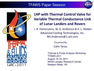
TFAWS Paper Session. Benchmarking of NX Space Systems Thermal (TMG) for use in Determining Specular Radiant Flux Distributions Carl Poplawsky (Maya Simulation Technologies) Dr. Chris Jackson (Maya Heat Transfer Technologies) Chris Blake (Maya Heat Transfer Technologies).

E N D
TFAWS Paper Session Benchmarking of NX Space Systems Thermal (TMG) for use inDetermining Specular Radiant Flux Distributions Carl Poplawsky (Maya Simulation Technologies)Dr. Chris Jackson (Maya Heat Transfer Technologies)Chris Blake (Maya Heat Transfer Technologies) Thermal & Fluids Analysis WorkshopTFAWS 2011August 15-19, 2011 NASA Langley Research CenterNewport News, VA
Agenda • Summary of NX Space Systems Thermal (NXSST) radiation calculation methods • Monte Carlo • Deterministic • Hemiview • Deterministic Benchmark for compound parabolic concentrator (CPC) Specular Reflection • Monte Carlo – reference solution • Deterministic - test analysis • Summary of diffuse/specular QA test results • Monte Carlo – reference solution • Deterministic - test analysis TFAWS 2011 – August 15-19, 2011
NXSST Radiation Calculation Methods • NX Space Systems Thermal (NXSST) includes three approaches for view factor calculations • Monte Carlo • Suitable for both diffuse and specular problems • Deterministic • Suitable for both diffuse and specular problems • Hemiview • Suitable only for diffuse problems • NXSST also has several choices for radiative conductance calculations • Monte Carlo • Gebhardt’s • Openheim’s TFAWS 2011 – August 15-19, 2011
NXSST Radiation Calculation Methods FEM Deterministic Ray Tracing/ Semi-Analytic Hemicube Monte Carlo Monte Carlo Geometric/Ray-Traced View Factors Radiosity (or Oppenheim’s) Method Gebhardt’s Method Radiative couplings (RAD-K’s) Numerical Model Other inputs (heat loads other conductances, etc.) Nonlinear outer iterations, linear solver Temperatures
NXSST Ray Tracing • Ray tracing enables treatment of optical properties beyond simple diffuse (Lambertian) emission and reflection • More complicated reflection and transmission optical properties can be supported if ray tracing is also introduced • Specular reflection from curved surfaces can be captured through use of parabolic shell elements • Ray tracing can be used in two ways: • With the Monte Carlo method, to compute heat loads and radiative exchange factors directly • To produce Ray-traced view factors with the Deterministic Method which can be used together with the view factor method
Ray Tracing With Monte Carlo • Monte Carlo ray-tracing can be used to compute view factors • More powerful is the application of Monte Carlo to compute radiativeconductances and radiative heat loads directly • This is the default behavior • Works by following the actual path of the radiation as it goes through the model • Instead of computing View Factors, MC computes the Gray Body View Factor: it is the fraction of energy leaving element i, absorbed by element j, including all intermediate reflections • Instead of computing radiative heat load view factors, Monte Carlo computes heat loads directly
NXSST Deterministic View Factor Method • For each element pair (i,j): • Determine if elements i,j are potentially shadowed • If not shadowed and target is diffuse • Compute view factor with exact contour integral method • If shadowed or target has specular or transmissive properties • Subdivide elements according to element subdivision criterion • Determine shadowing between sub-elements • For unshadowed sub-element pairs, determine view factor contribution using Nusselt sphere method • if target element is specular or transparent, ray trace the reflected or transmitted component through the model • Add view factor contributions of sub-elements
Deterministic Ray-tracing for view factor correction • Ray-tracing corrects the geometric view factors to account for specular reflections and transmission • Rays are launched from every element which has a direct view of an element with specular reflectivity or transmissivity • Ray density is controlled by the user through the subdivision or error control • Default is 256 rays per element pair • With the Deterministic option, ray distribution is deterministic, not random • Elements are subdivided and rays are launched between the subelements • Diffuse reflections are still accounted for through Oppenheim’s or Gebhardt’smethod • Effective radiating areas and optical properties are modified after ray tracing to account for effects which have already been ray-traced
NX SST Hemicube Method • With the Hemicube method, a half cube is situated around the “emitter” element. • Each face of the cube is divided into pixels, each pixel having a known view factor contribution. • The image of the surrounding “receiver” elements is projected onto the hemicube.
NX SST Hemicube Method • The hemicube algorithm in NX Thermal uses the Open Graphics Library (OGL) to render scenes (either on GPU or CPU) • During the solve, the hemicube engine draws the scene of elements as seen from each element in the Radiation Request • The software post processes these images to determine the view factors • Potentially very fast • Accuracy depends upon: • The number of pixels used to draw the images • Resolution limit associated with the minimum view factor contribution of one pixel • Error due to sampling from discrete locations of the viewing element (addressed with subdivision criteria) • Supports only diffuse (Lambertian) optical properties
NXSST Radiative Conductances • Radiative couplings (RAD-K’s) take into account all reflections including diffuse reflections • Radiosity (Oppenheim’s) method: • Additional radiosity nodes are introduced into the model, view factors can be used directly to calculate radiative couplings • Gebhardt’s method: • Radiative couplings are computed by solving a linear system involving the view factors and the optical properties • Monte Carlo • Radiative couplings are computed directly by tracing rays through the model • Ray behaviour statistically follows exactly the (non-wave) behaviour of the light travelling through the system
Deterministic Ray Tracing • In computing solar view factors, NXSST automatically uses ray-tracing to model specular reflections and transmissions. • The ray-tracing operations are carried out after computing the solar view factors for all elements. • Rays are launched from all elements which have a non-zero solar view factor and a specular reflectivity or transmissivity component defined. • ray density is controlled by the element subdivision parameter. • anti-aliasing algorithm automatically increases the subdivision parameter for specular and/or transmissive elements • When used with the View Factor Method: • Rays are traced through the enclosure until one of the following conditions is satisfied: • the ray impinges a fully diffuse element • the ray’s magnitude is reduced to less than 0.1% of its original value • the ray has been traced through 100 reflections • Diffusely reflected fluxes are distributed through the model using the view factors
Deterministic Benchmark for CPC Specular Reflection • The CPC is a good test for specular reflectivity • Concentrates light at the CPC exit (detector location) when within the acceptance angle (ө) • Essentially traps all incoming light • Light distribution at detector varies with light incidence angle (ø) Incidence Angle (ø) TFAWS 2011 – August 15-19, 2011
Deterministic Benchmark for CPC Specular Reflection • The CPC is defined with an off-axis revolved parabola • The focal point moves with light incidence angle (ø) • Focal point is beyond the detector when ø = 0 • Focal point is at the detector edge when ø = ө/2 TFAWS 2011 – August 15-19, 2011
Deterministic Benchmark for CPC Specular Reflection • 5mm exit diameter CPC chosen for benchmark • 45 degree acceptance angle • 25 degree acceptance angle 25 degrees 45 degrees (same scale) TFAWS 2011 – August 15-19, 2011
Deterministic Benchmark for CPC Specular Reflection • Mesh size held constant • 1mm parabolic triangular shells for the reflector • .5mm parabolic triangular shells for the detector • Linear elements are unsuitable for curved surface specularity 25 degrees 45 degrees (same scale) TFAWS 2011 – August 15-19, 2011
Deterministic Benchmark for CPC Specular Reflection • Monte Carlo used for reference solution • Studies at ø = 0° shows little sensitivity of average flux value at the detector to the number of rays/element for this example • Higher sensitivity may be observed with other optical geometries • 2000 rays/element chosen for reference solution TFAWS 2011 – August 15-19, 2011
Deterministic Benchmark for CPC Specular Reflection • Deterministic test analysis average detector flux correlates well with reference solution • ø = 0 degrees • Little sensitivity to number of subdivisions for this example • Higher sensitivity may be observed with other optical geometries • Deterministic subdivision factor = 3 used for all subsequent analysis solutions TFAWS 2011 – August 15-19, 2011
Deterministic Benchmark for CPC Specular Reflection • Deterministic test analysis detector flux distribution correlates well with reference solution • 25 degree CPC • ø = 0 degrees REFERENCE DETERMINISTIC TFAWS 2011 – August 15-19, 2011
Deterministic Benchmark for CPC Specular Reflection • Deterministic test analysis detector flux distribution correlates well with reference solution • 45 degree CPC • ø = 0 degrees REFERENCE DETERMINISTIC TFAWS 2011 – August 15-19, 2011
Deterministic Benchmark for CPC Specular Reflection • Deterministic test analysis average detector flux over a range of incidence angles correlates well with reference solution • ø = 0 to 30 degrees TFAWS 2011 – August 15-19, 2011
Deterministic Benchmark for CPC Specular Reflection • Deterministic test analysis detector flux distribution correlates well with reference solution • 25 degree CPC and ø = 15° REFERENCE DETERMINISTIC TFAWS 2011 – August 15-19, 2011
Deterministic Benchmark for CPC Specular Reflection • Deterministic test analysis detector flux distribution correlates well with reference solution • 45 degree CPC and ø = 30° REFERENCE DETERMINISTIC TFAWS 2011 – August 15-19, 2011
Deterministic Benchmark for CPC Specular Reflection • The Deterministic method provided a slight advantage in terms of computer resource for this example • CPU times are for the full solve through temperatures • Both CPC’s solved in the same solution • Results will vary depending on subdivision factor (DT) or rays/element (MC) • Reasonable values were used for this benchmark CPU Seconds Incidence Angle TFAWS 2011 – August 15-19, 2011
Deterministic Benchmark for CPC Specular Reflection • Deterministic method specular results are indistinguishable from those for the Monte Carlo reference solution • For the settings chosen for this benchmark, Deterministic provides a slight advantage in reduced computer resource • Monte Carlo and Deterministic approaches are equally recommended for specularity TFAWS 2011 – August 15-19, 2011
Summary of diffuse/specular QA test results • Over 30 test cases for specular/diffuse radiation models are exercised during QA testing for all NXSST releases • Temperature results differences between Monte Carlo, Deterministic are routinely tabulated • Using MC as the reference solution and the latest software revision, the maximum difference in local temperature was tabulated for each case, and then normalized • Deterministic models run with default view factor error criterion • Element view factor sum +/- 2% • Average normalized maximum temperature difference between DT and MC was .79% • Well within the default view factor error criterion TFAWS 2011 – August 15-19, 2011
NX Space Systems Thermal THANK YOU (www.mayahtt.com) TFAWS 2011 – August 15-19, 2011
CPC with Specular and Diffuse Properties • Mesh size held constant • 1mm linear triangular shells for the reflector • .5mm linear triangular shells for the detector • Linear elements chosen for the sake of speed 25 degrees Reflector Surface Properties εIR = 0.5 ρIR,d = 0.5 αS= 0 ρS,d = 0.5 ρS,s = 0.5 Detector Surface Properties εIR = 1 αS= 1 TFAWS 2011 – August 15-19, 2011
CPC with Specular and Diffuse Properties • Radiation problem setup • Conductive properties set to null; radiative problem only • Collimated solar flux of 1000 W/m2 parallel to CPC axis • Radiative heat exchange within the CPC and to the environment. No external radiation. • Two analysis types • Monte Carlo to compute RadKs and to compute heat loads • Deterministic to compute view factors with ray tracing; Oppenheim method for “RadKs”. Error criterion of 2%. • Parameters varied • Monte Carlo: # rays per element; same for radiation request and solar load calculations TFAWS 2011 – August 15-19, 2011
CPC with Specular and Diffuse Properties • As number of rays per element increases, detector temperatures level off and approach temperatures obtained by deterministic method with error criterion of 2% (dotted line) TFAWS 2011 – August 15-19, 2011
CPC with Specular and Diffuse Properties • Detector temperature distribution for deterministic case (error criterion 2%) correlates with Monte Carlo case (15000 rays/element) • Deterministic results are ~2.5% warmer MONTE CARLO DETERMINISTIC TFAWS 2011 – August 15-19, 2011
CPC with Specular and Diffuse Properties • Detector flux distribution for deterministic case (error criterion 2%) correlates well with Monte Carlo case (15000 rays/element) MONTE CARLO DETERMINISTIC TFAWS 2011 – August 15-19, 2011