Download

1 / 62
620 likes | 626 Views
RMP Coring Plans 2010 and Onward. RMP CFWG Meeting June 2009. Core- What Is It Good For?. Bay pollutant inventory erosional time bombs? Model validation Conceptual &/or mechanistic Model development Empirical, mechanistic, hybrid Can recalibrate, but better up front.

E N D
RMP Coring Plans 2010 and Onward RMP CFWG Meeting June 2009
Core- What Is It Good For? • Bay pollutant inventory • erosional time bombs? • Model validation • Conceptual &/or mechanistic • Model development • Empirical, mechanistic, hybrid • Can recalibrate, but better up front
Approach RMP/CEP 2006 • Select RMP S&T (random) and continuous (undiked) wetland sites • Vibracore in Bay, Livingstone (piston) core in wetlands/watershed • Freeze long core sections in field • Saw core into 2.5cm sections • Analyze sections at ~15 year intervals Using prelim. radiodating, literature estimates
RMP/CEP Sites (Bay) • Representative • inventory, sedimentation • 3 sites Central Bay, 2 sites each other segments • Preference to RMP repeat stations
Distribution of Sites (Wetland) • Loading history • Depositional zones • 1 site each segment • Pt Edith Martinez • Wildcat Richmond • Damon Sl. Oakland • Greco Island • Coyote Creek • +1 watershed site • Alviso Marina
Lessons RMP/CEP 2006 • Waiting for preliminary radiodating slowed study • 17 cores x 10 sections/core = 170 samples • Created backlog at RMP laboratories (3+ years equivalent of S&T samples) • Total cost $300k+, hard to reduce, especially analytical costs (1 site = 10 samples x X analytes)
Conceptual Model Sedimentation (from isotopes, bathymetric history) Similar in segment (shared water, sediment) But mesoscale differences (trib/shore proximity, etc) Pollutant distribution function of Sedimentation history Local land use/ loading
Bay Hg Results < 1960 < 1960 < 1960 < 1960 < 1960 < 1960 < 1960 < 1960
Conceptual Model Fits • Radiodating fits bathymetric history • North Bay erosive (137Cs, 210Pb near surface) • Central, South Bay ~neutral, or erosive • Lower South Bay depositional • Contamination fits sediment history • Top core sections ~ RMP surface sediments • Lower contamination in deepest sections • pre industrial background • Contaminants elevated in industrial period • Metals ~uniform downcore, PCBs higher nearer surface
Wetland Hg Results < 1960 < 1960 < 1960 < 1960 < 1960
Wetland Results • Radiodating fits sea level rise • All areas net depositional (2-3mm/year) • Lower South Bay subsiding, higher deposition • Contamination fits sediment history • Top core sections ~ RMP surface sediments • Usually lower contamination in deepest sections • pre industrial background • Contaminants elevated in industrial period • Sharper/higher peaks than in Bay cores • Watershed (Alviso) site ambiguous • Rapid deposition, but where is Hg peak?
Need Cores? • Better than before, but enough? • N = 11 from RMP/CEP + 2-5 from USGS • N depends on which analytes • Maybe OK for Baywide scale but not enough for segment specific modeling (N=2) • Time frame needed • Before models need new data • Resolution needed
Option 1: Repeat 2006 Effort • 10-11 RMP S&T (random) sites, 5 wetland, all Bay segments • Gravity/hammer core in Bay, Livingstone (piston) core in wetland • Freeze/saw subsampling 2.5cm sections • Analyze up to 10 sections at ~10cm (skipping) intervals (150-165 samples) PCBs, PBDEs, metals, TOC, grainsize • Total cost $350k+ ($300k in 2006)
Option 2: Incremental Efforts • 2 RMP S&T (random) sites (optionally +1 wetland?) in one Bay segment per year • Gravity/hammer core in Bay, Livingstone (piston) core in wetland • Freeze/saw subsampling into 2.5cm sections • Analyze up to 10 sections at ~10cm (skipping) intervals PCBs, PBDEs, metals, TOC, grainsize • Cost ~$50k for Bay cores, ~$75 w/ wetland
+/- Incremental Approach • Few sites, more often (e.g. 2 per segment, yearly) + Better workload for labs (20+ vs 100+ samples at once) + Costs better spread for RMP + Can get info on segments w/ greatest data needs first • Long time to get full Baywide set • Other details can be decided depending on program needs
Back to Basic Questions • Do we need more cores? • Probably, especially if we plan sub-segment scale models • All at once, or a few at a time? • A few at a time is easier for many logistical and budget reasons • When, where, how many? • Best early/before models finished, random/ representative of areas modeled, # samples depending on model Q’s
Nitty Gritty Details • Example design to follow if desired
Siting Approach 2010+ • Use new random RMP S&T sites + Continue to build larger scale spatial data ± May get stations w/ similar characteristics - Low odds for special sites of interest (hot spots, watershed deltas, dep/erosional
Sampling Approach 2010+ • Unpowered (push/gravity/hammer) cores + Low equipment needs/cost • Cores >1m deep may be difficult
Sectioning Approach 2010+ • Field freezing, saw sectioning + Easy sectioning post sampling (solid core) + No hold time issues (within ~1 year) • Freezing causes core distortion • Clean (e.g. Teflon) saw difficult/impossible, but the devil we know • (Alternatively) Field or lab extrusion + No freezing needed (~ambient or cooler chilling) ± Cleanliness unknown, depends on execution (staff, location, equipment) • Need extruding equipment/attachments
Analysis Approach 2010+ • Select set interval subsamples + Know which sections to send to labs a priori + Results from radiodating/chem labs sooner • Less flexibility on section spacing (longer or shorter cores, fast/slow deposition areas) ± (alternatively wait for radiodating, irregular spacing) • Skip sections + No need to composite 1 sample = 1 section, • May miss narrow peaks (how likely?) ± (alternatively composite sections)
Analysis Approach 2010+ • Analyte selection- highest needs for particle associated persistent pollutants of concern • PCBs • Hg • PBDEs (top 5 sections each core) • ??? • Add geologic /anthropogenic factors • ICP-MS trace elements • TOC, grainsize
Approach 2010+ Summary • 2 RMP S&T (random) sites (optionally +1 wetland?) in one Bay segment per year • Gravity/hammer core in Bay, Livingstone (piston) core in wetland • Freeze/saw subsampling into 2.5cm sections • Analyze up to 10 sections at ~10cm (skipping) intervals PCBs, PBDEs, metals, TOC, grainsize • Cost ~$50k for Bay cores, ~$75 w/ wetland
Dating: Bathymetric History (USGS Bruce Jaffe) Sum bathymetric changes between surveys + deposition – erosion Some sites depositional & erosional different periods
Dating: Isotopes (USC Hammond) Cs in A-bomb max ~1960 Pb decay half life 22 yrs Decay/ mixing dilution can look similar If Cs & Pb similar likely mixing dilution
LSB001: Fast accumulation ~150cm to 1960 ~60cm to 1960
LSB002: Fast accumulation ~130cm to 1960 ~30cm to 1960
LSB Wetland Deposition ~80cm to 1960
Hg Analyses • ICP-MS HF extract (CCSF) vs CVAFS aqua regia (MLML)
LSB Metals • Downcore concentrations noisy • Coyote Creek Hg max > Alviso! • Coyote Hg max @ 1960s depth (80cm) • Coyote Cu max @ 40cm = 1980s? • ~max Cu discharge late 1970s (Palo Alto) • ~surface sediment Cu USGS long term data
Conaway 2004 vs Current 5nmol/g ~ 1mg/kg
Lower South Bay PCBs • PCB in bay cores max subsurface • LSB001 max @40cm (60cm =1960) • LSB002 max @30cm (30cm = 1960)
SB001: Continuous Erosion? ~0cm to 1960 ~15cm to 1960 Core ID: SB001, X: 564867.30345800000, Y: 4163027.61900000000 1858 depth: -122 1898 depth: -123 1931 depth: -157 1956 depth: -124 1983 depth: -146 2005 depth: -160 2006 depth: -161 Reconstructed horizons: 0
SB002: No Change ~1950s ~0cm to 1960 ~12cm to 1960
SB Wetland Deposition ~30cm to 1960
South Bay Metals • Downcore concentrations noisy • Cu max @ Greco Island similar to Coyote, but into 1960s zone. • Greco Hg max ~uniform in wetland to 55cm = 1930s? (1960s Cs penetration to 30cm)
South Bay1960 = 12-15cm bay, 30cm wetland • PCB in bay max near surface • SB001 (continuous erosion) at top ~5cm • SB002 (no change since 1950s) ~10cm
CB001: No Change ~1940s ~0cm to 1960 ~5cm to 1960
CB002: Erosion to ~1920s ~0cm to 1960 ~20cm to 1960
CB006: Continuous Erosion ~0cm to 1960 ~12cm to 1960 Core ID: CB006A, X: 566290.21976900000, Y: 4174242.03589000000 1858 depth: -106 1898 depth: -134 1931 depth: -132 1956 depth: -183 1983 depth: -220 Reconstructed horizons: 0
Central Bay Metals • Bay downcore concentrations smaller range than in SB/LSB • No dating for wetland cores yet • ~20cm subsurface max for Hg, Se, Cu in wetland, • Similarly high conc for Se, Cu @ surface, 60cm
Central Bay PCBs1960 = 5-20cm bay, ?? wetland • PCB in bay max near surface • CB sites no change or eroding
SPB001: Erosion to ~1920s ~0cm to 1960 ~5cm to 1960
SPB002: Erosion to ~1880s ~0cm to 1960 ~2cm to 1960
San Pablo Metals • ~20cm surbsurface max for Hg, Se, Cu in wetland • No dating for wetland cores yet • No secondary metal peaks • Deeper concentrations fairly constant