Download
1 / 66
680 likes | 872 Views
Perturbations and Stability of Higher-Dimensional Black Holes. Hideo Kodama Cosmophysics Group Institute of Particle and Nuclear Studies KEK. Lecture at 4 th Aegean Summer School, 17-22 September 2007. Contents. Introduction Overview of the BH stability issue Linear perturbations

E N D
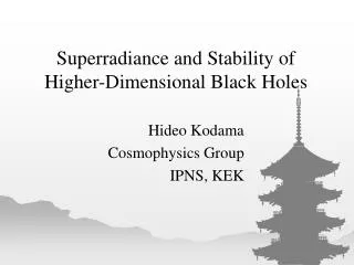
Perturbations and Stability of Higher-Dimensional Black Holes Hideo Kodama Cosmophysics Group Institute of Particle and Nuclear Studies KEK Lecture at 4th Aegean Summer School, 17-22 September 2007
Contents • Introduction • Overview of the BH stability issue • Linear perturbations • Perturbations of Static Black Holes • Background solution • Tensor/Vector/Scalar perturbations • Summary • Applications to Other Systems • Flat black branes • Rotating black holes • Accelerated black hole
Present Status of the BH Stability Issue Four-Dimensional Black Holes • Stable • Static black holes • Schwarzschild black hole [Vishveshwara 1970; Price 1972; Wald 1979,1980] • Reissner-Nordstrom black hole [Chandrasekhar 1983] • AdS/dS (charged) black holes [Ishibashi, Kodama 2003, 2004] • Skyrme black hole (non-unique system) [Heusler, Droz, Straumann 1991,1992; Heusler, Straumann, Zhou 1993] • Kerr black hole [Whiting 1989] • Unstable • YM black hole (non-unique system) [Straumann, Zhou 1990; Bizon 1991; Zhou, Straumann 1991] • Kerr-AdS black hole (l h <1, rh¿l) [Cardsoso, Dias, Yoshida 2006] • Unknown • Kerr-Newman black hole • Conjecture: large Kerr-AdS black holes are stable, but small ones are SR unstable [Hawking, Reall 1999; Cardoso, Dias 2004]
Higher-Dimensional Black Objects • Stable • Static black holes • AF vacuum static (Schwarzschild-Tangherlini) [Ishibashi, Kodama 2003] • AF charged static (D=5,6-11) [Kodama, Ishibashi 2004; Konoplya, Zhidenko 2007] • dS vacuum static (D=5,6,7-11), dS charged static (D=5,6-11) [IK 2003, KI 2004;Konoplya, Zhidenko 2007] • BPS charged black branes (in type II SUGRA) [Gregory, Laflamme 1994:Hirayama, Kang, Lee 2003] • Unstable • Static black string (in AdS bulk), black branes (non-BPS) [Gregory, Laflamme 1993, 1995; Gregory 2000; Hirayama, Kang 2001: Hirayama, Kang, Lee 2003; Kang; Seahra, Clarkson, Maartens 2005; Kudoh 2006] • Rapidly rotating special GLPP (Kerr-AdS) bh [Kunhuri, Lucietti, Reall 2006] • Unknown • Static black holes • AF charged static (D>11), AdS (charged) static (D>4), dS (charged) static (D>11) • Rotating black holes/rings • Conjecture: • Black rings are GL unstable. • Rapidly rotating MP black holes are GL unstable [Emparan, Myers 2003] • Doubly spinning black rings are SR unstable [Dias 2006] • Kerr black brane Kerr4£ Rp is SR unstable [Cardoso, Yoshida 2005]
Linear Perturbations Perturbation equations When the spacetime metric (and matter fields/variables) is expressed as the sum of a background part and a small deviation as in terms of the variables the linearlised Einstein equations can be written as where ML is the Lichnerowicz operator defined by
Linear Perturbations Gauge problems • Gauge freedom In order to describe the spacetime structure and matter configuration as a perturbation from a fixed background (M,g,), we introduce a mapping and define perturbation variables on the fixed background spacetime as follows: F
Gauge Problems • For a different mapping F', these perturbation variables change their values, which has no physical meaning and can be regarded as a kind of gauge freedom. • The corresponding changes of the variables are identical to the transformation of the variables with respect to the transformation f=F‘ -1F. In the framework of linear perturbation theory, • To be explicit,
Gauge Problems • Two methods to remove the gauge freedom • Gauge fixing method This method is direct, but it is rather difficult to find relations between perturbation variables in different gauges in general. • Gauge-invariant method This method describe the theory only in terms of gauge-invariant quantities. Such quantities have non-local expressions in terms of the original perturbation variables in general. These two approaches are mathematically equivalent, and a gauge-invariant variable can be regarded as some perturbation variable in some special gauge in general. Therefore, the non-locally of the gauge-invariant variables implies that the relation of two different gauges are non-local.
Gauge Problems • Harmonic gauge In this gauge, the perturbation equations read and the gauge transformation is represented as This gauge has residual gauge freedom • Synchronous gauge In the synchronous gauge in which there exist the residual gauge freedom given by For example, in the cosmological background this produces a suprious decaying mode represented by
Background Solution Ansatz • Spacetime • Metric where dn2=ij dxidxj is an n-dimensional Einstein space Kn satisfying the condition • Energy-momentum tensor
Background Solution Einstein equations • Notations • Einstein tensors • Einstein equations
Background Solutions Examples • Robertson-Walker universe: m=1 and K is a constant curvature space. • Brane-world model: m=2 (and K is a constant curvature space). For example, the metric of AdSn+2 spacetime can be written • HD static Einstein black holes: m=2 and K is an Einstein space. K=Sn for the Schwarzschild-Tanghelini black hole. In general, the generalised Birkhoff theorem says that the electrovac solutions satisfying the ansataz with m=2 are exhausted by the Nariai-type solutions and the black hole type solution
Examples • Black branes: m=2+k and K=Einstain space. In this case, the spacetime factor Nm is the product of a two-dimensional black hole sector and a k-dimensional brane sector: One can also generalise this background to introducing a warp factor in front of the black hole metric part. • HD rotating black hole (a special Myers-Perry solution):m=4 and K=Sn where all the metric coefficients are functions only of r and . • Axisymmetric spacetime: m is general and n=1.
Perturbations Gauge transformations For the infinitesimal gauge transformation the metric perturbation hMN= gMN transforms as and the energy-momentum perturbation MN= TMN transforms as
Perturbations Tensorial Decomposition • Algebraic tensorial type • Spatial scalar: hab, ab • Spatial vector: hai, ai • Spatial tensor: hij, ij • Decomposition of vectors A vector field vi on K can be decomposed as • Decomposition of tensors Any symmetric 2-tensor field on K can be decomposed as
Tensorial Decopositions • Irreducible types • In the linearised Einstein equations, through the covariant differentiation and tensor-algebraic operations, quantities of different algebraic tensorial types can appear in each equation. • However, in the case in which Kn is a constant curvature space, perturbation variables belonging to different irreducible tensorial types do not couple in the linearised Einstein equations, because there exists no quantity of the vector or the tensor type in the background except for the metric tensor. • The same result holds even in the case in which Kn is an Einstein space with non-constant curvature, because the only non-trivial background tensor other than the metric is the Weyl tensor that can only tranform a 2nd rank tensor to a 2nd rank tensor.
Tensor Perturbations Tensor Harmonics • Definition where the Lichnerowitcz operator on K is defined by When K is a constant curvature space, this operator is related to the Laplace-Beltrami operator by Hence, Tiijsatisfies We use k2 in the meaning of L-2nKfrom now on when K is an Einstein space with non-constant sectional curvature.
Tensor Harmonics • Properties • Identities: For any symmetric 2-tensor on a constant curvature space satisfying the following identities hold: • Spectrum: Let Mn be a n-dimensional constant curvature compact space with sectional curvature K. Then, the spectrum of k2 for the symmetric rank 2 harmonic tensor satisfies the condition • Sn: k2=l(l+n-1)-2, l=2,3,.. • 2-dim case • In this case, a tensor hamonic represents an infinitesimal deformation of the moduli parameters. • In particular, there exists no tensor harmonics on S2.
Tensor Perturbations Perturbation Equations • Harmonic expansion • Gauge-invariant variables • Einstein Equations Only the (i,j)-component of the Einstein equations has the tensor-type component: Here, ¤=DaDa is the D'Alembertian in the m-dimensional spacetime N.
Tensor Perturbations Applications to the static Einstein black hole • Master Equation A static Einstein black hole corresponds to the case m=2 and For this background, the perturbation equation without source which can be written where
Applications to a Static BH • Stability • For the Schwarzschild black hole, we can show that Vt¸0. Hence, it is stable. However, Vtis not positive definite in general, and the stability is not so obvious. • Energy integral From the equation for HT, we find Hence, in the case K is a constant curvature space, the stability of tensor perturbations results from k2¸n|K|,
Vector Perturbations Vector Harmonics • Definitions Harmonic tensors Exceptional modes: The following harmonic vectors correspond to the Killing vectors and are exceptional:
Vector Harmonics • Properties • Spectrum: From the identities We obtain the general bound the spectrum • Sn: k2=l(l+n-1)-1, l=1,2,… • Exceptional modes: The exceptional modes exist only for K¸0. For K=0, such modes exist only when K is isomorphic to TN£ Cn-N, where Cn-N is a Ricci flat space with no Killing vector.
Vector Perturbation Perturbation equations • Harmonic expansion • Gauge transformations For the vector-type gauge transformation the perturbation variables transform as • Gauge invariants
Perturbation equations • Einstein equations • Generic modes • Exceptional mode:k2=(n-1)K(¸0)
Vector Perturbation Codimension Two Case • Master equation • Generic modes From the energy-momentum conservation, one of the perturbation equation can be written This leads to the master variable in terms of which the remaining perturbation equation can be written • Exceptional modes
Codimension Two Case • Static black hole • Master equation where This equation is identical to the Regge-Wheeler equation for n=2, K=1 and =0.
Codimension Two Case • Potentials
Codimension Two Case • Stability • In the 4D case with n=2, K=1, =0, we have • In higher-dimensional cases, although the potential becomes negative near the horizon, we can prove the stability in terms of the energy integral because mv¸0:
Scalar Perturbations Scalar Harmonics • Definition • Harmonic vectors • Harmonic tensors • Exceptional modes
Scalar Harmonics • Properties • Spectrum: For Qijdefined by We have the identity From this we obtain the following bound on the spectrum • For Sn: k2= l(l+n-1), l=0,1,2,…
Scalar Perturbation Linear Perturbations • Harmonic expansion • Gauge transformations For the scalar-type gauge transformation the perturbation variables transform as
Linear Perturbations • Gauge invariants From the gauge transformation law we find the following gauge-invariant combinations.
Linear Perturbations • Einstein equations • Gab :
Linear Perturbations • Gai : • Tracefree part of Gij : • Gii:
Scalar Perturbation Codimension Two Case • Master equation For a static Einstein black hole, in terms of the master variable the perturbation equations for a scalar perturbation can be reduced to where
Codimension Two Case • Potentials
Codimension Two Case • Stability • For n=2, K=1, =0, the master equation coincides with the Zerilli equation and the potential is obviously positive definite: where m=(l-1)(l+2). • In higher dimensions, we have an conserved energy integral, • We cannot conclude stability using this integral because Vs is not positive definite in general.
Codimension Two Case • S-deformation • Let us deform the energy integral with the help of partial integrations as where Then, the effective potential changes to • For example, for we obtain where
Flat Black Branes • ASS4Lecture.dvi
Rotating Black Holes • Simple AdS-Kerr: a1=a, a2=…=aN=0 • In this case, the metric is U(1)£ SO(n+1) symmetric with n=D-4. • For D¸ 7, the harmonic amplitude HT for tensor-type metric perturbations obeys the equation This equation is exactly identical to the equation for the harmonic amplitude for a minimally-coupled massless scalar field in the same background! Therefore, we can apply the results on stability/instability of a massless scalar field to the tensor modes. • In particular, we can conclude that tensor perturbations are stable for a2l2 < rh4 on the basis of the argument by Hawking, Reall 1999.
Slowly Rotating AdS-Kerr • Everywhere Time-like Killing Vector For slowly rotating black hole, there exists a Killing vector that is everywhere timelike in DOC: for example, when ai2 l2< rh4 (i=1,2) for D=5, or when a12l2< rh4, a2=…=aN=0. • Energy Conservation Law In this case, no instability occurs for a matter field satisfying the dominant energy condition [Hawking, Reall 1999] where n T k is non-negative everywhere on . • Stability Conjecture On the basis of this observation, Hawking and Reall conjectured that AdS-Kerr black holes with slow rotations such that ai2 l2< rh4 will be stable against gravitational perturbations as well. At the same time, they also conjecture that rapidly rotating AdS-Kerr black holes will be unstable. This conjecture was proved for D=4 and rh¿l[Cardoso, Dias, Yoshida 2006]
Energy Integral for Tensor Perturbations of Simple AdS-Kerr: In the coordinates in which the metric is written for (t,r,x) defined by the following energy integral is conserved: where , F and U0 are always positive outside horizon, while U1 is positive definite only for a2l 2 < rh4.
Effective Potential • In the effective potential both U0 and U1 are positive for a2l 2 < rh4. • For a2l 2 > rh4 , however, U1 becomes negative in some range of r at x=-1, and the negative dip of the potential becomes arbitrarily deep as m increases. • Hence, it is highly probable that simple AdS-Kerr black holes in dimensions higher than 6 are unstable for tensor perturbations. • If we take ! 0 ( l !1) limit with fixed a and rh, the above stability condition is violated. This may suggest the instability of MP black holes unless the growth rate of instability vanishes at this limit.
Equally Rotating AdS-Kerr: a1==aN=a with D=2N+1. • In this case, the angular part of the metric has the structure of a twisted S1 bundle over CPN-1. • For a special class of tensor perturbations, the metric perturbation equation can be reduced to a Schrodinger-type ODE that has the same structure as that for a massless free scalar field. • It is claimed on the basis of analysis utilising the WKB approximation that such tensor perturbations satisfying the “superradiant condition”=m h are unstable if hl > 1, i.e., if there does not exist a global timelike Killing vector. [Kunhuri, Lucietti, Reall 2006]
Accelerated Black Hole C-metirc • Metric C-metric is a Petrov type D static axisymmetric vacuum solution to the Einstein equations with cosmological constant. The special case of the most general type D electrovac solution by Plebanski JF, Demianski M 1976