Download

1 / 16
160 likes | 271 Views
CS 290H 26 October Sparse approximate inverses, support graphs. Homework 2 due Mon 7 Nov. Sparse approximate inverse preconditioners Introduction to support theory. Preconditioned conjugate gradient iteration. x 0 = 0, r 0 = b, d 0 = B -1 r 0, y 0 = B -1 r 0

E N D
CS 290H 26 OctoberSparse approximate inverses, support graphs • Homework 2 due Mon 7 Nov. • Sparse approximate inverse preconditioners • Introduction to support theory
Preconditioned conjugate gradient iteration x0 = 0, r0 = b, d0 = B-1r0, y0 = B-1r0 for k = 1, 2, 3, . . . αk = (yTk-1rk-1) / (dTk-1Adk-1) step length xk = xk-1 + αk dk-1 approx solution rk = rk-1 – αk Adk-1 residual yk = B-1rk preconditioning solve βk = (yTk rk) / (yTk-1rk-1) improvement dk = yk + βk dk-1 search direction • Several vector inner products per iteration (easy to parallelize) • One matrix-vector multiplication per iteration (medium to parallelize) • One solve with preconditioner per iteration (hard to parallelize)
A B-1 Sparse approximate inverses • Compute B-1 A explicitly • Minimize || A B-1 – I ||F (in parallel, by columns) • Variants: factored form of B-1, more fill, . . • Good: very parallel, seldom breaks down • Bad: effectiveness varies widely
Support Graph Preconditioning • CFIM: Complete factorization of incomplete matrix • Define a preconditioner B for matrix A • Explicitly compute the factorization B = LU • Choose nonzero structure of B to make factoring cheap (using combinatorial tools from direct methods) • Prove bounds on condition number using both algebraic and combinatorial tools +: New analytic tools, some new preconditioners +: Can use existing direct-methods software -: Current theory and techniques limited
Some classes of matrices • Diagonally dominant symmetric positive definite: • Diagonally dominant M-matrix: • Laplacian: • Generalized Laplacian:
3 7 1 3 7 1 6 8 6 8 4 10 4 10 9 2 9 2 5 5 Combinatorial half: Graphs and sparse Cholesky Fill:new nonzeros in factor Symmetric Gaussian elimination: for j = 1 to n add edges between j’s higher-numbered neighbors G+(A)[chordal] G(A)
Spanning Tree Preconditioner [Vaidya] • A is symmetric positive definite with negative off-diagonal nzs • B is a maximum-weight spanning tree for A (with diagonal modified to preserve row sums) • factor B in O(n) space and O(n) time • applying the preconditioner costs O(n) time per iteration G(A) G(B)
Numerical half: Support numbers Intuition from resistive networks:How much must you amplify B to provide the conductivity of A? • The support of B for A is σ(A, B) = min{τ : xT(tB– A)x 0 for all x, all t τ} • In the SPD case, σ(A, B) = max{λ : Ax = λBx} = λmax(A, B) • Theorem:If A, B are SPD then κ(B-1A) = σ(A, B) · σ(B, A)
Splitting Lemma • Split A = A1+ A2 + ··· + Ak and B = B1+ B2 + ··· + Bk • Ai and Bi are positive semidefinite • Typically they correspond to pieces of the graphs of A and B (edge, path, small subgraph) • Lemma: σ(A, B) maxi {σ(Ai , Bi)}
Spanning Tree Preconditioner [Vaidya] • A is symmetric positive definite with negative off-diagonal nzs • B is a maximum-weight spanning tree for A (with diagonal modified to preserve row sums) • factor B in O(n) space and O(n) time • applying the preconditioner costs O(n) time per iteration G(A) G(B)
Spanning Tree Preconditioner [Vaidya] • support each edge of A by a path in B • dilation(A edge) = length of supporting path in B • congestion(B edge) = # of supported A edges • p = max congestion, q = max dilation • condition number κ(B-1A) bounded by p·q (at most O(n2)) G(A) G(B)
Spanning Tree Preconditioner [Vaidya] • can improve congestion and dilation by adding a few strategically chosen edges to B • cost of factor+solve is O(n1.75), or O(n1.2) if A is planar • in experiments by Chen & Toledo, often better than drop-tolerance MIC for 2D problems, but not for 3D. G(A) G(B)
Splitting and Congestion/Dilation Lemmas • Split A = A1+ A2 + ··· + Ak and B = B1+ B2 + ··· + Bk • Ai and Bi are positive semidefinite • Typically they correspond to pieces of the graphs of A and B (edge, path, small subgraph) • Lemma: σ(A, B) maxi {σ(Ai , Bi)} • Lemma: σ(edge, path) (worst weight ratio) · (path length) • In the MST case: • Ai is an edge and Bi is a path, to give σ(A, B) p·q • Bi is an edge and Ai is the same edge, to give σ(B, A) 1
Algebraic framework • The support of B for A is σ(A, B) = min{τ : xT(tB– A)x 0 for all x, all t τ} • In the SPD case, σ(A, B) = max{λ : Ax = λBx} = λmax(A, B) • If A, B are SPD then κ(B-1A) = σ(A, B) · σ(B, A) • [Boman/Hendrickson] If V·W=U, then σ(U·UT, V·VT) ||W||22
Algebraic framework [Boman/Hendrickson] Lemma: If V·W=U, then σ(U·UT, V·VT) ||W||22 Proof: • take t ||W||22 = λmax(W·WT) = max y0 { yTW·WTy / yTy } • then yT (tI - W·WT) y 0 for all y • letting y = VTx gives xT (tV·VT - U·UT) x 0 for all x • recall σ(A, B) = min{τ : xT(tB– A)x 0 for all x, all t τ} • thus σ(U·UT, V·VT) ||W||22
[ ] a2 +b2-a2 -b2 -a2 a2 +c2 -c2-b2 -c2 b2 +c2 [ ] a2 +b2-a2 -b2 -a2 a2 -b2 b2 B =VVT A =UUT ] [ ] ] [ [ 1-c/a1 c/b/b ab-a c-b ab-a c-b-c = x U V W -a2 -c2 -a2 -b2 -b2 σ(A, B) ||W||22 ||W||x ||W||1 = (max row sum) x (max col sum) (max congestion) x (max dilation)