Download
1 / 24
270 likes | 431 Views
Weighted Importance Sampling Techniques for Monte Carlo Radiosity. Ph. Bekaert, M. Sbert, Y. Willems Department of Computer Science, K.U.Leuven I.M.A., U.d.Girona. Overview. Weighted Importance Sampling = Biased but consistent generalization of importance sampling

E N D
Weighted Importance Sampling Techniques forMonte Carlo Radiosity Ph. Bekaert, M. Sbert, Y. Willems Department of Computer Science, K.U.Leuven I.M.A., U.d.Girona
Overview • Weighted Importance Sampling = Biased but consistent generalization of importance sampling • Application to Form Factor Integration • Application to Stochastic Jacobi Radiosity
Uniform Sampling • xi chosen uniformly • scores have equal weights 1/N • unbiased
Importance Sampling • xi sampled non-uniformly (pdf q) • scores have equal weights 1/N
Importance Sampling • xi sampled non-uniformly • scores have equal weights • better if pdf matches function more closely • pdf must be practical
Weighted Uniform Sampling • xi sampled uniformly • non-uniform weights wi compensate for not sampling p • Also perfect if p matches f • Powell&Swann’66
Weighted Importance Sampling • xi sampled according to source pdf q • non-uniform weights wi compensate for not sampling the target pdf p • Spanier’79
Weighted Importance Sampling • A-posteriori correction to Importance Sampling: • Compare MSE: • Bias vanishes rapidly with N:
Global vs Local Weighting Characteristic function • Consider sub-domain: • Global weighting: Correction factor depends on all samples in D, is the same for every sub-interval and is little effective.
Global vs Local Weighting Characteristic function • Consider sub-domain: • Global weighting: • Local Weighting: Correction factor depends only on samples in sub-domain. normalized restriction of p and q to sub-domain
Form Factor Integration • Sample points x on S1 uniformly: • 3 strategies to sample points y on S2: • (A) Uniform Area Sampling. • (B) Uniform Direction Sampling (Arvo’95). • (C) Cosine-distributed Direction Sampling. • Mimic (C) using (A): Low Variance in spite of uniform area sampling
Form Factor Integration: Results Infinite variance!! About as good as or even a little bit better than uniform direction sampling
Form Factor Integration: Results Some bias at low nr of samples
Jacobi Iterative Method • Power equations: • Deterministic Jacobi Algorithm: (quadratic cost)
Stochastic Jacobi Iterations A) Local Lines 1) Select patch j: 2) Select i conditional on j: 3) Score (form factor cancels!!) VARIANCE: (log-linear cost)
1) Select patch j and i: B) Global Lines 2) Score Higher variance per sample, but cheaper samples.
Global Weighting • Mimic local lines with cheaper global lines: Problem: same correction factor for all patches + depends on all samples.
Per-patch (local) Weighting • Normalization of target pdf required, so can only use global line pdf as target: • When is weighting better? Compare estimates for M.S.E.: • Decide a-posteriori whether to weight or not! • Low additional cost with M.S.E. weighting M.S.E. no weighting
Weighting reduces noise Without weighting With weighting 3250 patches about 250 rays per patch 30 seconds CPU time (195MHz R10k) Reflectivity about 70%
deep blue = 10 times better light blue = 3 times better green = neutral yellow = 3 times worse red = 10 times worse Speedup • predicted and observed speed-up correspond well • good prediction for reasonable number of samples, except on tiny patches. Predicted (1 run of 250 rays/patch) Observed (100 runs of 250 rpp) Predicted (1 run of 100,000 rpp)
Bias is not objectionable 250 rays/patch (100 runs) 100,000 rays per patch (1 run) (Highly exaggerated) High bias on tiny patches (very low nr. of samples) Bad meshing (shadow leak)
With hierarchical refinement • Without weighting: • High variance on small • elements created during • refinement • Shadow leak artifacts. With weighting: (solution based on the same samples!) Indirect illumination computed using stochastic Jacobi (2 min.) Direct illumination computed using stochastic ray tracing
Conclusion • Consistent generalization of importance sampling (a-posteriori correction) • Potentially high benefit (factor >10 in SJR) at very low additional cost • and if it doesn’t help it doesn’t harm either • Future Work: • benefit estimation for very low nr of samples • other applications.