Download
1 / 30
300 likes | 435 Views
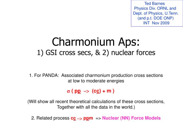
Ted Barnes Physics Div. ORNL and Dept. of Physics, U.Tenn. (and p.t. DOE ONP) INT Nov 2009. Charmonium Aps: 1) GSI cross secs, & 2) nuclear forces. 1. For PANDA: Associated charmonium production cross sections at low to moderate energies

E N D
Ted Barnes Physics Div. ORNL and Dept. of Physics, U.Tenn. (and p.t. DOE ONP) INT Nov 2009 Charmonium Aps:1) GSI cross secs, & 2) nuclear forces • 1. For PANDA: Associated charmonium production cross sections • at low to moderate energies • s( pp-> (cc) + m ) • (Will show all recent theoretical calculations of these cross sections, • Together with all the data in the world.) • 2. Related process cc-> ppm => Nuclear (NN) Force Models
1. What PANDA is all about: • The search for non-qq mesons. • To many theorists this suggests qq + gluonic excitation, • = “hybrid mesons”. • Smoking gun: hybrids can have all JPC, unlike qq. • Just search for a meson with JPC-exotic quantum numbers; • 0 - - ;1 - +,2 + -,3 - +,4 + -, … • Panda logic: • Light meson studies (u,d,s) were already well underway (prev. LEAR, BNL, JLAB), • How about going to heavy quarks? cc-hybrids? Narrower states, cleaner spectrum. • JPC-Exotic Charmonium hybrids = the ultimate goal of PANDA@GSI. • We already have the LEAR community (ca. 300 people). Let’s use pp.
Y(4415) cc-H ~ 4.3 [GeV] X(3872) J/Y(3097) PANDA at GSI…(ProtonAntiprotonaNnihilationexperimentatDArmstadt) p beam energies… KEp = 0.8 – 14.5 [GeV]: Allows access to cc and cc-H mass range. pp-> cc + m, cc-H + m “m” = light meson(s) Kinematics of pp-> cc + m s½ hc(2980)
something else e.g. typically p 0 p p qq quant. nos. only p p All JPC quant. nos., including cc-hybrids with exotic JPC Why associated production? (pp-> cc +m, (cc)H +m) Problem: You can’t make JPC-exotics in s-channel pp annihilation (as in E760/835 at Fermilab), since pp only accesses conventional meson (qq) quantum numbers. To make J PC- exotic hybrids you have to make something else to recoil against (associated production): New Problem: Just how big are these cross sections? Let’s look at all the world’s data.
s ( pp->p0 J/y ) E760 All the world’s (published) data on pp-> cc + meson (exclusive) processes. our calc. Evidently ca. 0.1–0.2 [nb] near threshold for J/y . Other states, other energies??? Nada. all the world’s data on s(pp-> mJ/y)
pp J/ + 0 from continuum Expt… Only 2 E760 points published. This is E835, c/o D.Bettoni. Physical cross sec is ca. 100x this. M. Andreotti et al., PRD 72, 032001(2005)
What PANDA needs to know: What are the approximate low-E cross sections for pp->Y+ meson(s) ? (Y is a generic charmonium or charmonium hybrid state.) Recoil against meson(s) allows access to JPC-exotic Y.
2. Theoretical estimates of low to moderate energy • associated charmonium cross sections • s ( pp->cc + m ) (What you can do in lieu of a direct measurement of these cross sections. Also includes other possible experiments.) The actual processes are obscure at the q+g level, so “microscopic” models will be problematic. We just need simple “semiquantitative” estimates. A quick run through the literature (just 4 references) …
Approximate low to moderate-E cross sections for pp-> Y + meson(s) = ? Four theor. references to date: 1. M.K.Gaillard. L.Maiani and R.Petronzio, PLB110, 489 (1982). PCAC W(q) (pp-> J/y + p 0 ) 2. A.Lundborg, T.Barnes and U.Wiedner, PRD73, 096003 (2006). Crossing estimates for s( pp-> Y m) from G( Y-> p p m) (Y = y, y‘ ; m = several) 3. T.Barnes and X.Li, hep-ph/0611340, PRD75, 054018 (2007). PCAC-like model W(q),s ( pp-> Y + p 0 ),Y = hc, y, c0, c1, y ‘ 4. T.Barnes, X.Li and W.Roberts, arXiv:0709.4491, PRD77, 056001 (2008). [3] model, e+e--> J/y-> pp (for BES), pp-> J/y + p 0 W and s. Dirac and Pauli strong ppJ/y FFs.Polarization.
1. M.K.Gaillard. L.Maiani and R.Petronzio, PLB110, 489 (1982). PCAC-like model W(q) (pp-> J/y + p 0 ) Soft Pion Emission in pp Resonance Formation Motivated by CERN experimental proposals (LEAR). Assumes low-E PCAC-like dynamics with the pp system in a definite J,S,L channel. (Hence not immediately useful for total cross section estimates for PANDA.) Quite numerical, gives W(q) at a specific Ep(cm) = 230 MeV as the only example. Implicit analytic results completed in Ref.2. “pion ISR”
2. A.Lundborg, T.Barnes and U.Wiedner, hep-ph/0507166, PRD73, 096003 (2006). “summer in Uppsala” Charmonium Production in pp Annihilation: Estimating cross sections from decay widths. Crossing estimates: We have experimental results for ca. 10decays of the type Y->ppm. These have the same amplitude as the desired s( pp-> Ym ). Given a sufficiently good understanding of the decay Dalitz plot, we can usefully extrapolate from the decay to the production cross section. n.b. Also completes the derivation of some implicit results for cross sections in the Gaillard et al. PCAC-like paper. 0th-order estimate: assume a constant amplitude, then s( pp-> Ym) is simply proportional to G(Y->ppm ). Specific example, s(pp-> J/y + p0 ):
we know … we want … p0 p0 p p J/y A A p p J/y These processes are actually not widely separated kinematically:
For a 0th-order (constant A) cross section estimate we can just swap 2-body and 3-body phase space to relate a generic cc s( pp->Yp0) toG( Y->ppp0 ) Result: where AD is the area of the decay Dalitz plot: Next, an example of the numerical cross sections predicted by this simple estimate, compared to the only (published) data on this type of reaction… s( pp->J/yp0)fromG( J/y->ppp0 ), compared to the E760 data points:
const. amp. model all the world’s published data (E760) our calc. Not bad for a first rough “phase space” estimate. Improved cross section estimates require a model of the reaction dynamics (next).
Before we proceed… The const. amp. approx. says other channels may be larger. This approx. however is very suspect. N* resonances?
3. T.Barnes and Xiaoguang Li, hep-ph/0611340; PRD75, 054018 (2007). “summer in Darmstadt” Associated Charmonium Production in Low Energy pp Annihilation Calculates the differential and total cross sections for pp-> Y + p 0 using the same PCAC-like model assumed earlier by Gaillard et al., but for incident pp plane waves, and several choices for Y: hc, J/y, c0, c1, y‘. The a priori unknown Ypp couplings are taken from the (now known) pp widths.
T.Barnes and X.Li, hep-ph/0611340; PRD75, 054018 (2007). gpg5 GY PCAC-like model of pp->Y + p0: Assume simple pointlike hadron vertices; gpg5 for the NNp vertex, GY = gY (g5, -i gm, -i, -i gmg5) for Y = (hc, J/y and y’, c0, c1) Use the 2 tree-level Feynman diagrams to evaluate ds/dt and s. +
mp = 0 limit, fairly simple analytic results… unpolarized differential cross sections: simplifications M = mY m = mp x = (t - m2) / m2 y = (u - m2) / m2 f = -(x+y) = (s - mp2 - M 2) / m2 r i = m i / m also, in both d<s>/dt and <s>, (in the analytic formulas)
mp = 0 limit, fairly simply analytic results… unpolarized total cross sections: (analytic formulas)
This is where it gets really interesting. However we would really prefer to give results for physical masses and thresholds. So, we have also derived the more complicated mp .ne. 0 formulas analytically. e.g. of the pp-> J/yp0 unpolarized total cross section: Values of the {appY} coupling constants?
gpg5 GY To predict numerical pp -> Y + p0 production cross sections in this model, we know gppp ~ 13.5 but not the { gppY }. Fortunately we can get these new coupling constants from the known Y-> pp partial widths: Our formulas for G( Y-> pp ): Resulting numerical values for the { gppY } coupling constants: (Uses PDG total widths and pp BFs.) !! !
s( pp->J/yp0), PCAC-like model versus “phase space” model: G(J/y-> pp) and gNNp=13.5 input “real dynamics” G(J/y-> p0pp) input “phase space”
Now we can calculate NUMERICAL total and differential cross sections for pp-> any of these cc states + p0. We can also answer the big question, Are any cc states produced more easily in pp than J/y? (i.e. with significantly larger cross sections than s ( pp -> J/yp0) )
And the big question… Are any other cc states more easily produced than J/y? ANS: Yes, by 1-2 orders of magnitude!
Final result for cross sections. (All on 1 plot.) Have also added two E835 points (open) from a PhD thesis.
An interesting observation: The differential cross sections have nontrivial angular dependence. e.g. This is the c.m. frame (and mp=0) angular distribution for pp->hcp0at Ecm = 3.5 GeV: beam axis Note the (state-dependent) node, at t = u. Clearly this and the results for other quantum numbers may have implications for PANDA event identification.
Predicted c.m. frame angular distribution for pp->hcp0 normalized to the forward intensity, for Ecm = 3.2 to 5.0 GeV by 0.2. spiderman plot
Predicted c.m. frame angular distribution for pp->J/yp0 normalized to the forward intensity, for Ecm = 3.4 to 5.0 GeV.