Download

1 / 8
80 likes | 221 Views
FP Fitting. Huanlong Liu. FP equation. where:. long time large energy barrier approximations:. dynamic time. energy barrier. overdrive (current and field). where: k is the switching rate. Switching rate @ long-time.

E N D
FP Fitting Huanlong Liu
FP equation where: • long time large energy barrier approximations: dynamic time energy barrier overdrive (current and field) where: k is the switching rate.
Switching rate @ long-time If we assume the dynamic time (τD), energy barrier (ξ) and zero-T critical current (Ic0) are the same, then the switching rate is only the function of current amplitude (I).
Overlay experimental data too long Fitting is done by using Eq. (1) with all free parameters. Plot in log(k) for clear observation
Other fitting parameters • In order to have reasonable dynamic time, we can reduce the number of free parameters inside Eq. (1). • These fits are done with fixed τD and Ic0 as inputs, only allow ξ to be free. • A reasonable energy barrier can be obtained. • However, Eq. (1) may not be able to fit all experimental data. • Larger τD and Ic0 lead to a better fit.
Fitting parameters • Energy barrier ξ, the free parameter obtained from the fit, plotted as a function of dynamic time τDand zero-T critical current Ic0, which are inputs and kept fixed for the fit. • From the range of reasonable τD and Ic0, we obtain a range of reasonable ξ. • In general, larger τD and Ic0 lead to smaller ξ as expected. • ξdepends more on Ic0 than τD, since Ic0 and ξ alone determines the slope of log(k) versus I, which shouldn’t vary much for a reasonable fit to experiments.
Fitting parameters II • r2 = sum[(log(k)exp – log(k)cal)2], where log(k)cal is calculated from Eq. (1) using the same fitting parameters (Ic0, ξandτD) as those in the previous slide with the same current (I) as those in experiments. • r2 indicates how good the fit is. • Better fit for larger τD and Ic0, yet most of them are reasonable. The worst is shown in slide 5 with τD = 0.1 ns and Ic0 = 6.0 mA. Next step:Can we find a set of parameters that also fits the short time data? We have reasonable fittings with a wide range of parameters for the long time data.
Finding Ic0 first • Calculate P versus τ using the same parameters (Ic0 = 6.8 mA, ξ = 164 andτD = 0.3 ns) for two currents and compare with experiments. • The FP calculation is faster than experiment for smaller I but slower for larger I, which indicates that Ic0 needs to be increased for the calculation. • Now I’m looking into larger Ic0s to see if I can get parameters that fit both long and short times.