Download
1 / 16
160 likes | 332 Views
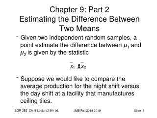
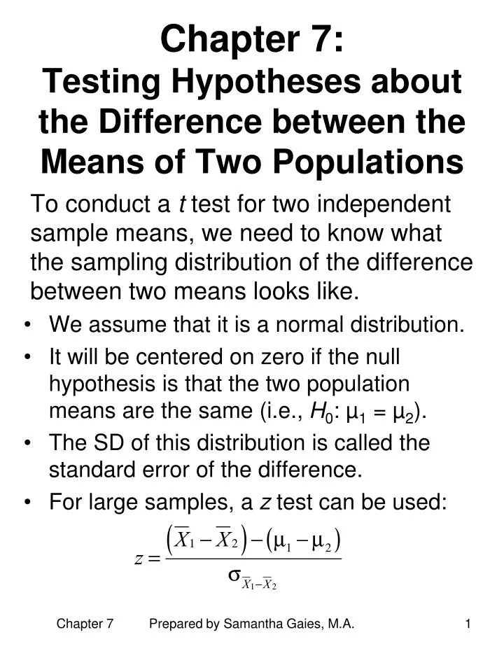
Chapter 7: Testing Hypotheses about the Difference between the Means of Two Populations. To conduct a t test for two independent sample means, we need to know what the sampling distribution of the difference between two means looks like. We assume that it is a normal distribution.

E N D
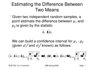
Chapter 7: Testing Hypotheses about the Difference between the Means of Two Populations To conduct a t test for two independent sample means, we need to know what the sampling distribution of the difference between two means looks like. • We assume that it is a normal distribution. • It will be centered on zero if the null hypothesis is that the two population means are the same (i.e., H0: µ1 = µ2). • The SD of this distribution is called the standard error of the difference. • For large samples, a z test can be used: Prepared by Samantha Gaies, M.A.
Estimating the Standard Error of the Difference When the Sample Sizes Are Not Large • Pooled-variances estimate: the two sample variances can be pooled together to form a single estimate of the population variance called s2pooled ors2p • s2pooled can then be used to estimate the standard error of the difference by using the following formula: • The use of s2p is based on the assump-tion that the two populations have the same variance. Prepared by Samantha Gaies, M.A.
The Pooled-Variances t Test Formula • The denominator of this formula is the estimated standard error of the difference (SED): • Inserting the formula for estimating the SED from the pooled variances yields the following formula: • Note that the use of s2pooled is based on the assumption that the two populations have the same variance and that df = N1 + N2 – 2. Prepared by Samantha Gaies, M.A.
Alternative Versions of the Pooled-Variances t Test Formula • Here, the formula for s2pooled is included in the t formula, and it is assumed that the null hypothesis is µ1 – µ2 = 0: where the critical t is based on df = N1 + N2 – 2 • The formula for equal sample sizes reduces to: where the critical t is based on df = 2n – 2. Prepared by Samantha Gaies, M.A.
Try this example: A researcher is studying the effect of drinking Red Bull on the number of errors a partici-pant makes in a motor skills test. Test the null hypothesis that the population mean for Red Bull drinkers is the same as for placebo drinkers. t.05 (32) = 2.04 (approx.) < 5.51, so the null hypothesis can be rejected. Prepared by Samantha Gaies, M.A.
Limitations of Statistical Conclusions • Our significant Red Bull result could be a Type I error. If this is a novel result, replication is recommended. • Statistical significance is no guarantee that you are dealing with a large or important difference. • If you have not assigned participants to the two conditions (e.g., you are comparing habitual coffee drinkers with those who do not like coffee), you cannot make causal conclusions from your significant results. • More information can be obtained by constructing a confidence interval for the difference of the means of the two populations. Prepared by Samantha Gaies, M.A.
Confidence Intervals for the Difference between Two Population Means • The formula for the CI for the difference of two population means is obtained by solving the t test formula for µ1 – µ2. • For a 95% CI, tcrit is the critical t for a .05, two-tailed significance test. For the Red Bull example, the 95% CI is: • Thus, the CI extends from a difference of 2.52 errors up to a difference of 5.48 errors. • Because zero is not in the interval, we know that the usual H0 can be rejected at the .05 level, with a two-tailed test. Prepared by Samantha Gaies, M.A.
Assumptions for the Two-Group t Test and CI for the Difference of Population Means • The dependent variable has been meas-ured on an interval or ratio scale (there are nonparametric tests available if an ordinal scale was used). • Independent Random Sampling • Ideal: both groups should be random samples. • Each individual selected for one sample should be independent of all the individuals in the other sample. • However, typically, the two groups are formed by random assignment from one sample of convenience. • Normal Distributions • The DV should follow a normal distribution in both groups. • However, the Central Limit Theorem implies that, if the samples are not very small, the two-group t test will still be valid. Prepared by Samantha Gaies, M.A.
Assumptions (cont.) • To use the pooled-variance t test, an additional assumption must be made: Homogeneity of Variance. • However, this assumption is usually ignored if: • both samples are quite large, or • the two samples are the same size, or • the sample variances are not very different (e.g., one variance is no more than twice as large as the other) • If it is not reasonable to assume HOV, consider performing the separate-variances t test: • The df for the critical t are best found by statistical software. Prepared by Samantha Gaies, M.A.
Measuring the Size of an Effect • A standardized effect-size measure, g, can be defined as: where sp is the square root of the pooled variance • Or, • If N1≠ N2, then use the harmonic mean of the sample sizes to obtain n for the preceding formula: Prepared by Samantha Gaies, M.A. .
The t Test for Matched Samples Let us begin with an example: A researcher is interested in whether students who study while watching TV devote as much attention to their studies as students who don’t watch TV. Fourteen students are matched on age, grades, and IQ, and then the students of each pair are randomly assigned to either watch TV while studying or not. The data below are the scores on a 10-point quiz based on the material the students were asked to study. Prepared by Samantha Gaies, M.A.
Null hypothesis: If TV has no effect, we would expect a mean difference of 0: H0: μD = 0;H1: μD ≠ 0 • The actual mean of the differences is ΣD / N = –10 / 7 = –1.43, and the variance of the differences is 1.95. • Calculating the matched t value: • The df for the critical tequals N – 1, where N equals the number of pairs. For this example, df = 7 – 1 = 6. • t.05 (6) = 2.447 < 2.71, so the null hypo-thesis can be rejected—watching TV seems to make a difference. Prepared by Samantha Gaies, M.A.
Confidence Interval for the Population Mean of Difference Scores: • Applied to the TV / No TV example, the 95% CI is: = –1.43 – 1.29 = – 2.72 Thus, the 95% CI goes from –.14 to –2.72. We can be 95% sure that TV watching reduces these quiz scores, relative to a control group, somewhere between .14 and 2.72 points. Recall that, because zero is not in the 95% CI, we know that we could reject the null hypoth-esis of no difference at the .05 level, two-tailed. Prepared by Samantha Gaies, M.A.
Comparing the t Test for Matched Pairs with the t Test for Independent Samples • The numerator remains the same. • The denominator is usually smaller for matched pairs; the better the matching, the smaller the denominator gets. • Fewer df for the matched t test means a larger critical value to beat, but the increase in the calculated t usually outweighs this drawback. Prepared by Samantha Gaies, M.A.
Types of Matched t Test Designs • Repeated Measures(i.e., same participants measured twice) • Simultaneous (e.g., mixed trials) • Successive: two subtypes: • Before-after (may lack control group) • Counterbalanced • Deals well with simple order effects (e.g., practice and fatigue) • Cannot eliminate differentialcarryover effects, in which case a matched-pairs design may be superior (see next slide) Prepared by Samantha Gaies, M.A.
Types of Matched t Test Designs (cont.) • Matched-Pairs (i.e., different participants with something in common) • Experimental • Pairs are created through a relevant pretest or available data • Pairs may act as “judges” and rate the same set of stimuli • Natural • Uses naturally occurring pairs (e.g., husbands and wives, siblings) • Need to be especially cautious about conclusions because the experimenter did not create the pairings Prepared by Samantha Gaies, M.A.