Download
1 / 33

E N D
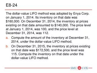
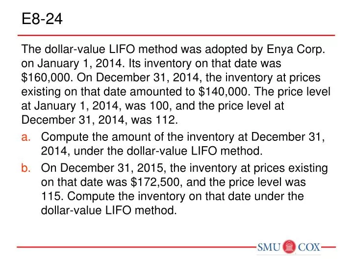
E8-24 The dollar-value LIFO method was adopted by Enya Corp. on January 1, 2014. Its inventory on that date was $160,000. On December 31, 2014, the inventory at prices existing on that date amounted to $140,000. The price level at January 1, 2014, was 100, and the price level at December 31, 2014, was 112. • Compute the amount of the inventory at December 31, 2014, under the dollar-value LIFO method. • On December 31, 2015, the inventory at prices existing on that date was $172,500, and the price level was 115. Compute the inventory on that date under the dollar-value LIFO method.
E8-24 a. Adjust 2014 inventory to 2013 base-year prices: $140,000 / 1.12 = $125,000 Calculate current year LIFO layer: $125,000 – $160,000 = ($35,000) Layer liquidation Calculate LIFO layers at end of period prices: $125,000 * 1.00 = $125,000
E8-24 b. Adjust 2015 inventory to 2013 base-year prices: $172,500 / 1.15 = $150,000 Calculate current year LIFO layer: $150,000 – $125,000 = $25,000 Layer Calculate LIFO layers at end of period prices: $125,000 * 1.00 = $125,000 25,000 * 1.15 = 28,750 $153,750
LCM Practice Decker Company has five products in its inventory. Information about the December 31, 2011, inventory follows. Unit Unit Unit Replacement Selling ProductQuantityCostCostPrice A 1,000 $10 $12 $16 B 800 15 11 18 C 600 3 2 8 D 200 7 4 6 E 600 14 12 13 The selling cost for each product consists of a 15 percent sales commission. The normal profit percentage for each product is 40 percent of the selling price. Determine the balance sheet inventory carrying value at December 31, 2011, assuming the LCM rule is applied to individual products.
LCM Practice Decker Company has five products in its inventory. Information about the December 31, 2011, inventory follows. Unit Unit Unit Replacement Selling ProductQuantityCostCostPrice A 1,000 $10 $12 $16 B 800 15 11 18 C 600 3 2 8 D 200 7 4 6 E 600 14 12 13 The selling cost for each product consists of a 15 percent sales commission. The normal profit percentage for each product is 40 percent of the selling price. Determine the balance sheet inventory carrying value at December 31, 2011, assuming the LCM rule is applied to individual products.
LCM Practice Decker Company has five products in its inventory. Information about the December 31, 2011, inventory follows. Unit Unit Unit Replacement Selling ProductQuantityCostCostPrice A 1,000 $10 $12 $16 B 800 15 11 18 C 600 3 2 8 D 200 7 4 6 E 600 14 12 13 The selling cost for each product consists of a 15 percent sales commission. The normal profit percentage for each product is 40 percent of the selling price. Determine the balance sheet inventory carrying value at December 31, 2011, assuming the LCM rule is applied to the entire inventory.
LCM Practice Inventory carrying value would be $30,390, the lower of aggregate inventory cost ($33,600) and aggregate inventory market ($30,390). The amount of the loss from inventory write-down is $3,210 ($33,600 – 30,390). Journal entry to write-down would be: COGS (or Loss Due to Decline in Inventory) 3,210 Inventory 3,210 Don’t worry about the idea of an Allowance related to LCM
Practice: Conventional Retail Method Smith-Kline Company maintains inventory records at selling prices as well as at cost. For 2011, the records indicate the following data: Cost Retail Beginning inventory $ 80 $ 125 Purchases 671 1,006 Freight-in on purchases 30 Purchase returns 1 2 Net markups 4 Net markdowns 8 Net sales 916 Use the conventional retail method to approximate cost of ending inventory.
Practice: (Conventional Retail) Cost Retail Beginning inventory $ 80 $ 125 Purchases 671 1,006 Freight-in on purchases 30 Purchase returns (1) (2) Net markups 4 Goods available for sale 780 1,133 Cost-to-retail percentages: Conventional cost ratio: $780 / $1,133 = 0.6884 Deduct: Net sales (916) Net markdowns (8) Ending inventory at retail $ 209 Ending inv at cost($209 x .6884) $144
LIFO to FIFO Conversion – Dow Chemical LIFO FIFO 6,847+ 818= 7,665 6,847 46,020 46,020 52,867 53,685 45,595 7,087+ 1,003= 8,090 7,087 45,780
E9-12 Astaire Company uses the gross profit method to estimate inventory for monthly reporting purposes. Presented below is information for the month of May. Inventory, May 1 $ 160,000 Purchases (gross) 640,000 Freight-in30,000 Sales1,000,000 Sales returns 70,000 Purchase discounts 12,000 • Compute the estimated inventory at May 31, assuming that the gross profit is 25% of sales. • Compute the estimated inventory at May 31, assuming that the gross profit is 25% of cost.
E9-12(a) Inventory, May 1 $ 160,000 Purchases (gross) 640,000 Freight-in30,000 Sales1,000,000 Sales returns 70,000 Purchase discounts 12,000 • Compute the estimated inventory at May 31, assuming that the gross profit is 25% of sales.
E9-12(a) Inventory, May 1 $ 160,000 Purchases (gross) 640,000 Freight-in30,000 Sales1,000,000 Sales returns 70,000 Purchase discounts 12,000 • Compute the estimated inventory at May 31, assuming that the gross profit is 25% of sales.
E9-12(a) Inventory, May 1 $ 160,000 Purchases (gross) 640,000 Freight-in30,000 Sales1,000,000 Sales returns 70,000 Purchase discounts 12,000 • Compute the estimated inventory at May 31, assuming that the gross profit is 25% of sales.
E9-12(a) Inventory, May 1 $ 160,000 Purchases (gross) 640,000 Freight-in30,000 Sales1,000,000 Sales returns 70,000 Purchase discounts 12,000 • Compute the estimated inventory at May 31, assuming that the gross profit is 25% of sales.
E9-12(b) • Compute the estimated inventory at May 31, assuming that the gross profit is 25% of cost. Not the easiest to use since we don’t know cost! GP = COGS * 25% and Sales – COGS = GP GP = (Sales – GP) * 25% GP = Sales * 25% – GP *25% GP + GP * 25% = Sales * 25% GP * 125% = Sales * 25% GP = Sales * 25% / 125% GP = Sales * 20%
E9-12(b) Inventory, May 1 $ 160,000 Purchases (gross) 640,000 Freight-in30,000 Sales1,000,000 Sales returns 70,000 Purchase discounts 12,000 • Compute the estimated inventory at May 31, assuming that the gross profit is 25% of cost (i.e., 20% of sales).
E9-12(b) Inventory, May 1 $ 160,000 Purchases (gross) 640,000 Freight-in30,000 Sales1,000,000 Sales returns 70,000 Purchase discounts 12,000 • Compute the estimated inventory at May 31, assuming that the gross profit is 25% of cost (i.e., 20% of sales).
E10-25 On April 1, 2012, Pavlova Company received a condemnation award of $410,000 cash as compensation for the forced sale of the company’s land and building, which stood in the path of a new state highway. The land and building cost $60,000 and $280,000, respectively, when they were acquired. At April 1, 2012, the accumulated depreciation relating to the building amounted to $160,000. On August 1, 2012, Pavlova purchased a piece of replacement property for cash. The new land cost $90,000, and the new building cost $380,000. Prepare the journal entries to record the transactions on April 1 and August 1, 2012.
E10-25: Continued April 1 Cash410,000 Accumulated Depreciation—Buildings 160,000 Land 60,000 Buildings 280,000 Gain on Disposal of Plant Assets 230,000 August 1 Land 90,000 Buildings 380,000 Cash 470,000
Example 9 On January 1, 2011, the Haskins Company adopted the dollar-value LIFO method for its one inventory pool. The pool’s value on this date was $660,000. The 2011 and 2012 ending inventory valued at year-end costs were $690,000 and $760,000, respectively. The appropriate cost indexes are 1.04 for 2011 and 1.08 for 2012. Calculate the inventory value at the end of 2011 and 2012 using the dollar-value LIFO method.
Example 9: Continued 2011 Ending Inventory at Base Year Cost $690,000 / 1.04 = $663,462 Inventory Layers at Base Year Cost Base$660,000 2011 3,462 $663,462 Inventory Layers Converted to Cost $660,000 x 1.00 = $660,000 3,462 x 1.04 = 3,600 $663,600
Example 9 On January 1, 2011, the Haskins Company adopted the dollar-value LIFO method for its one inventory pool. The pool’s value on this date was $660,000. The 2011 and 2012 ending inventory valued at year-end costs were $690,000 and $760,000, respectively. The appropriate cost indexes are 1.04 for 2011 and 1.08 for 2012. Calculate the inventory value at the end of 2011 and 2012 using the dollar-value LIFO method.
Example 9: Continued 2012 Ending Inventory at Base Year Cost $760,000 / 1.08 = $703,704 Inventory Layers at Base Year Cost Base$660,000 2011 3,462 2012 40,242 $703,704 Inventory Layers Converted to Cost $660,000 x 1.00 = $660,000 3,462 x 1.04 = 3,600 40,242 x 1.08 = 43,461 $707,061
Example 10 Mercury Company has only one inventory pool. On December 31, 2011, Mercury adopted the dollar-value LIFO inventory method. The inventory on that date using the dollar-value LIFO method was $200,000. Inventory data are as follows: Ending Inventory at Ending Inventory at Year Year-End Costs Base Year Costs 2012 $231,000 $220,000 2013 299,000 260,000 2014 300,000 250,000 Compute the inventory at December 31, 2012, 2013, and 2014, using the dollar-value LIFO method.
Example 10: Continued 2012 Calculation of Cost Index $231,000 / $220,000 = 1.05 Inventory Layers Converted to Cost $200,000 x 1.00 = $200,000 20,000 x 1.05 = 21,000 $221,000
Example 10: Continued 2013 Calculation of Cost Index $299,000 / $260,000 = 1.15 Inventory Layers Converted to Cost $200,000 x 1.00 = $200,000 20,000 x 1.05 = 21,000 40,000 x 1.15 = 46,000 $267,000
Example 10 Mercury Company has only one inventory pool. On December 31, 2011, Mercury adopted the dollar-value LIFO inventory method. The inventory on that date using the dollar-value LIFO method was $200,000. Inventory data are as follows: Ending Inventory at Ending Inventory at Year Year-End Costs Base Year Costs 2012 $231,000 $220,000 2013 299,000 260,000 2014 300,000 250,000 Compute the inventory at December 31, 2012, 2013, and 2014, using the dollar-value LIFO method.
Example 10: Continued 2014 Calculation of Cost Index $300,000 / $250,000 = 1.20 Inventory Layers Converted to Cost $200,000 x 1.00 = $200,000 20,000 x 1.05 = 21,000 30,000 x 1.15 = 34,500 $255,500
E9-24(a) You assemble the following information for Dillon Department Store, which computes its inventory under the dollar-value LIFO method. Cost Retail Inventory on January 1, 2012 $222,000 $300,000 Purchases 364,800 480,000 Increase in price level for year 9% Compute the cost of the inventory on December 31, 2012, assuming that the inventory at retail is $294,300. • Beginning cost-to-retail = 222,000 / 300,000 = 74% • Current cost-to-retail = 364,800 / 480,000 = 76% • Ending inventory at base year cost is 294,300 / 1.09 = 270,000 • Since less than the 300,000 beginning retail (at base year cost) there is no new layer created and entire inventory will be at beginning cost-to-retail and beginning price index (=1.00) • 270,000 * 74% * 1.00 = 199,800
E9-24(b) You assemble the following information for Dillon Department Store, which computes its inventory under the dollar-value LIFO method. Cost Retail Inventory on January 1, 2012 $222,000 $300,000 Purchases 364,800 480,000 Increase in price level for year 9% Compute the cost of the inventory on December 31, 2012, assuming that the inventory at retail is $359,700. • Beginning cost-to-retail = 222,000 / 300,000 = 74% • Current cost-to-retail = 364,800 / 480,000 = 76% • Ending inventory at base year cost is 359,700 / 1.09 = 330,000 • Since more than the 300,000 beginning retail (at base year cost) there is a new layer created • 300,000 * 74% * 1.00 = 222,000 30,000 * 76% * 1.09 = 24,852 330,000246,852