Download

1 / 13
130 likes | 239 Views
Unit 1: Functions and Models Part 3: Linear Regression. Lines of Best Fit. The sum of squared residuals can be used to determine which of two lines is the better fit to a set of data. In some cases, this is rather straightforward. In other cases, you may have to try several lines.

E N D
Lines of Best Fit • The sum of squared residuals can be used to determine which of two lines is the better fit to a set of data. • In some cases, this is rather straightforward. • In other cases, you may have to try several lines. • The line of best fit, also known as the least squares line or regression line, has three important properties: • It is the line that minimizes the sum of squared residuals, and it is unique. There is only one line of best fit for a set of data. • It contains the center of mass of the data, that is, the point, () whose coordinates are the mean of the x-values and the mean of the y-values. • Its slope and intercept can be computed directly from the coordinates of the given data points. • NOTE: The formula for the slope of the least squares line is too complex for computation by hand. Each statistics utility has a regression routine that will take the coordinates of a set of data points and compute the slope and y-intercept of the line of best fit.
Example • Heavy metals can enter the food chain when metal-rich discharges from mines contaminate streams, rivers, and lakes. The table shows the lead and zinc contents in milligram of metal per kilogram of fish (mg/kg) for 10 whole fish (4 rainbow trout, 4 large scale suckers, and 2 mountain whitefish) taken from the Spokane River during July, August, and October of 1999. • Use a statistics utility to find an equation of the least squares line to predict the amount of zinc from the amount of lead.
Example • Use a statistics utility to find an equation of the least squares line to predict the amount of zinc from the amount of lead. • Find the center of mass. Is it on the line? • Find the sum of the squared residuals for the regression.
Example • Use a statistics utility to find an equation of the least squares line to predict the amount of lead from the amount of zinc. • Find the center of mass. Is it on the line? • Find the sum of the squared residuals for the regression.
Example • Are your two answers the same? • Use an appropriate equation to predict the amount of zinc in a fish that has 2 mg/kg of lead.
Correlation • To measure the strength of the linear relation between two variables, a correlation coefficient is used. • Denoted by the letter ‘r’.
Correlation • Unlike the sum of the squared residuals, which can be measured for any line modeling a set of data, the correlation coefficient describes the fit and direction for the regression line only. • It can be proved that, regardless of the data set, the correlation coefficient, r, is always between -1 and 1. Some data sets and the corresponding values of ‘r’ are shown.
Correlation • The sign of ‘r’ indicates the direction of the relation between variables, and the magnitude indicates the strength of the relation. • Positive values of ‘r’ indicate a positive association between the variables, • That is, larger values of one variable are associated with larger values of the other. • Negative values of ‘r’ indicate a negative association between variables • Larger values of one variable are associated with smaller values of the other. • The extreme values of 1 and -1 indicate a perfect linear relation, as in scatter plots A and D in the previous example. • This means that all data lies on a line. • Also known as a perfect correlation.
Correlation • A relation for which most data fall close to a line is called a strong correlation. • A weak correlation is one for which, although a linear trend can still be seen, many points are not very close to the line. • A value of ‘r’ close to or equal to zero indicates that the variables are not related by a linear model. • Note that the variables may be related in some other way as denoted by the pattern. • There are no strict rules about how large a correlation value must be to be considered strong.
Activity • Why is the correlation coefficient 1 for Set 1? • The x- and y- values in Sets 3 and 4 are swapped. How does this affect ‘r’? Does this make sense? • The line of best fit for Set 5 has a slope of 0 and an ‘r’ value of 0. However, there is a definitive pattern. What other type of model would fit these data?
Correlation • Some statistic utilities give values of r2 instead of r. • This is because r2 is used in advanced statistical techniques. • You can calculate ‘r’ by taking the square root of this value, and determine the sign of the correlation according to the direction of the scatter plot.
Cautions about Correlation! • While ‘r’ provides a mathematical measure of linearity, it does not provide information about cause and effect. • Ex: There is a large positive correlation between shoe size and reading level of children, but this does not necessarily mean that learning to read better causes your feet to grow or that wearing bigger shoes improves your reading. • It is still up to people to analyze and interpret data to understand why two variables might be related. • This can be summarized as “correlation does not imply causation”. • Watch out for influential points. Outliers can have a strong impact on the values of slope, y-intercept, and correlation on the least squares line.