Download
1 / 20
200 likes | 202 Views
This figure displays various climate anomalies in the Niño-3.4 region, including sea surface temperature (SST), ocean temperature, wind, and circulation patterns. The anomalies are departures from the 1971-2000 baseline period means.

E N D
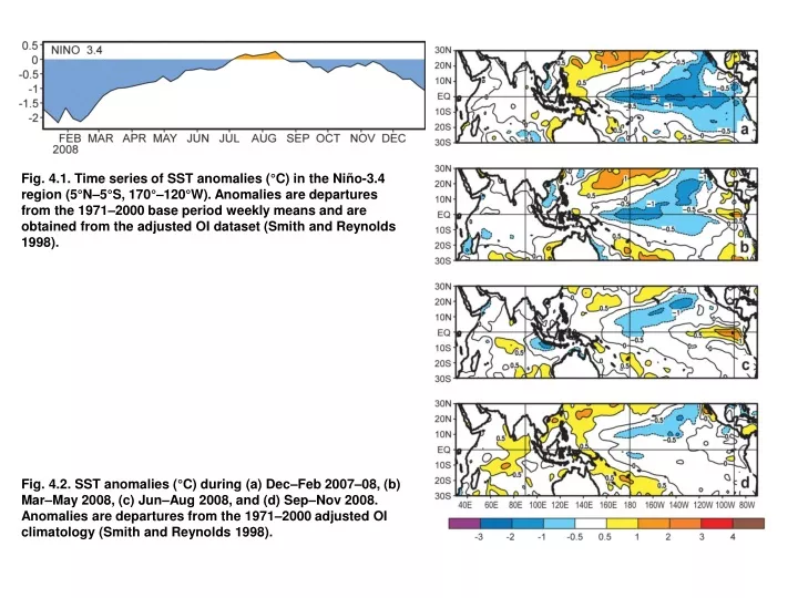
Fig. 4.1. Time series of SST anomalies (°C) in the Niño-3.4 region (5°N–5°S, 170°–120°W). Anomalies are departures from the 1971–2000 base period weekly means and are obtained from the adjusted OI dataset (Smith and Reynolds 1998). Fig. 4.2. SST anomalies (°C) during (a) Dec–Feb 2007–08, (b) Mar–May 2008, (c) Jun–Aug 2008, and (d) Sep–Nov 2008. Anomalies are departures from the 1971–2000 adjusted OI climatology (Smith and Reynolds 1998).
Fig. 4.3. Equatorial depth-longitude section of ocean temperature anomalies (°C) averaged between 5°N and 5°S during (a) Dec–Feb 2007–08, (b) Mar–May 2008, (c) Jun–Aug 2008, and (d) Sep–Nov 2008. The 20°C isotherm (thick solid line) approximates the center of the oceanic thermocline. The data are derived from an analysis system that assimilates oceanic observations into an oceanic GCM (Behringer et al. 1998). Anomalies are departures from the 1971–2000 period monthly means. Fig. 4.4. Anomalous 850-hPa wind vector and speed (m s−1) and anomalous OLR (shaded, W m−2) during (a) Dec–Feb 2007–08, (b) Mar–May 2008, (c) Jun–Aug 2008, and (d) Sep–Nov 2008. Anomalies are departures from the 1979–95 period monthly means.
Fig. 4.5. 200-hPa circulation during Dec 2007–May 2008: (a) anomalous streamfunction (shading) and vector winds (m s−1) and (b) total streamfunction (contours) and wind speed (shading). In (a), anomalous ridges are indicated by positive values (red) in the NH and negative values (blue) in the SH. Anomalous troughs are indicated by negative values in the NH and positive values in the SH. In (b), “L” indicates mid-Pacific trough and “H” indicates western Pacific subtropical ridge. Anomalies are departures from the 1971–2000 period monthly means. Fig. 4.6. Time–longitude section of filtered 200-hPa velocity potential anomaly (5°N–5°S) for 2008. Green (brown) shading represents anomalous divergence (convergence). Red lines highlight the MJO signal. The three MJO episodes are marked. Anomalies are departures from the 1971–2000 base period daily means.
Fig. 4.8. ACE values expressed as percent of the 1950–2000 median value (87.5 × 10⁴ kt2). ACE is a wind energy index that measures the combined strength and duration of the NSs. ACE is calculated by summing the squares of the 6-hourly maximum sustained surface wind speed in knots (Vmax2) for all periods while the storm has at least TS strength. Pink, yellow, and blue shades correspond to NOAA’s classifications for above-, near-, and below-normal seasons, respectively. Fig. 4.7. Time–longitude section of the upper ocean (0–300 m) heat content anomaly (5°N–5°S) for 2008. Blue (yellow/red) shading indicates below- (above) average heat content. The downwelling phases (solid lines) of oceanic Kelvin waves are indicated. Anomalies are departures from the 1982–2004 base period pentad means.
Fig. 4.9 (a) SST anomalies (°C) during Aug–Oct 2008. (b) Consecutive Aug–Oct area-averaged SST anomalies in the MDR. Red line shows the corresponding 5-yr running mean. Green box in (a) denotes the MDR. Anomalies are departures from the 1971–2000 monthly means.
Fig. 4.10. Aug–Oct 2008: (a) total CAPE (J kg−1) and anomalous vector winds (m s−1) at 10 m; (b) anomalous sea level pressure (shading, hPa) and vector winds at 10 m; (c) 700-hPa anomalous cyclonic relative vorticity (shading) and vector winds, with thick arrow indicating the observed AEJ core; (d) 200-hPa anomalous heights and vector winds. Green boxes denote the MDR. Anomalies are departures from the 1971–2000 monthly means.
Fig. 4.12. 200-hPa velocity potential (shading) and divergent wind vectors (m s−1): (a) Aug–Oct 2008 anomalies and (b) high-activity (1995–2008) period means minus low-activity (1971–94) period means. Anomalies are departures from the 1971–2000 monthly means. Fig. 4.11. Aug–Oct 2008: 200–850-hPa vertical wind shear magnitude (m s−1) and vectors (a) total and (b) anomalies. In (a), shading indicates values below 8 m s−1. In (b), red (blue) shading indicates below- (above) average magnitude of the vertical shear. Green boxes denote the MDR. Anomalies are departures from the 1971–2000 monthly means.
Fig. 4.14. 200-hPa streamfunction (shading) and vector wind (m s−1): (a) Aug–Oct 2008 anomalies and (b) high-activity (1995–2008) period means minus low-activity (1971–94) period means. In (a), anomalous ridges are indicated by positive values (red) in the NH and negative values (blue) in the SH. Anomalous troughs are indicated by negative values in the NH and positive values in the SH. Anomalies are departures from the 1971–2000 monthly means. Fig. 4.13. Time series showing consecutive Aug–Oct values of area-averaged (a) 200–850-hPa vertical shear of the zonal wind (m s−1), (b) 700-hPa zonal wind (m s−1), and (c) 700-Pa relative vorticity (× 10−6 s−1). Blue curves show unsmoothed values, and red curves show a 5-pt running mean of the time series. Averaging regions are shown in the insets.
Fig. 4.15. Apr–Jun 2008 anomalies at 200 hPa: (a) velocity potential (shading) and divergent wind vectors (m s−1) and (b) streamfunction and total wind vectors (m s−1). In (b), anomalous ridges are indicated by positive values (red) in the NH and negative values (blue) in the SH. Anomalous troughs are indicated by negative values in the NH and positive values in the SH. Anomalies are departures from the 1971–2000 monthly means. Fig. 4.16. Seasonal TC statistics for the east North Pacific Ocean during 1970–2008: (a) number of NS, H, and MH and (b) ACE (× 104 kt2) with the seasonal total for 2008 highlighted in red. Both time series include the 1971–2005 base period means.
Fig. 4.17. The 200–850-hPa vertical wind shear anomaly (m s−1) during (top) Jun–Aug and (bottom) Sep–Nov 2008. Anomalies are departures from the 1979–2004 period means. (Source: NOAA NOMADS NARR dataset.)
Fig. 4.18. (a) Number of TSs, TYs, and STYs per year in the WNP 1945–2008. (b) Cumulative number of TCs with TS intensity or higher (NS) per month in the WNP: 2008 (black line) and climatology (1971–2000) shown as box plots [interquartile range: box, median; red line, mean; blue asterisk, values in the top or bottom quartile; blue crosses, high (low) records in the 1945–2006 period; red diamonds (circles)]. (c) Number of NSs per month in 2008 (black curve); mean climatological number of NSs per month (blue curve); the blue plus signs denote the maximum and minimum monthly historical values (1945–2008); and green error bars show the interquartile range for each month. In the case of no error bars, the upper and/or lower percentiles coincide with the median. (d) Cumulative number of TYs per month in the western North Pacific: 2008 (black line) and climatology (1971–2000) shown as box plots. (e) Number of TYs per month in 2008 (black curve); mean climatological number of TY per month (blue curve); the blue plus signs denote the maximum and minimum monthly historical values (1945–2008); and green error bars show the interquartile range for each month. (Source: 1945–2007 JTWC best-track dataset, 2008 JTWC preliminary operational track data.)
Fig. 4.19. (a) ACE values per year in the WNP for 1945–2008. The solid green line indicates the median for 1971–2000 climatology, and the dashed green lines show the 25th and 75th percentiles. (b) ACE values per month in 2008 (red line) and the median in 1971–2000 (blue line), where the green error bars indicate the 25th and 75th percentiles. In the case of no error bars, the upper and/or lower percentiles coincide with the median. The blue plus signs denote the maximum and minimum values during the period 1945–2008. (Source: 1945–2007 JTWC best-track dataset, 2008 JTWC preliminary operational track data.) Fig. 4.20. (a) Zonal 850-hPa winds (m s−1) from JASO 2008. The contour interval is 1 m s−1. (b) Genesis potential index (Camargo et al. 2007b) anomalies for JASO 2008. (Source: atmospheric variables—NCEP reanalysis data; Kalnay et al. 1996; SST—Smith and Reynolds 2005.)
Fig. 4.21. Annual TC statistics for the NIO over the period 1970–2008: (a) number of TSs, CYCs, and MCYCs, and (b) the estimated annual ACE (× 104 kt2) for all TCs during which they were at least TS or greater intensities (Bell et al. 2000). The 1981–2005 base period means are included in both (a) and (b). Note that the ACE values are estimated due to a lack of consistent 6-h-sustained winds for every storm Fig. 4.22. Same as in Fig. 4.21, but for TCs in the SIO over the period 1980–2008.
Fig. 4.23. TC frequencies in the southwest Pacific, 1976–2008. Fig. 4.24. TC tracks in the Southwest Pacific, 2007–08.
Fig. 4.25. Annual average rainfall rate from TRMM 0.25° analysis for (top) Jan 2008 and (bottom) May 2008. Note the uneven contour intervals (0.5, 1, 2, 4, 6, 8, 10, 15, and 20 mm day−1). Fig. 4.26. Latitudinal cross-sections of TRMM rainfall (mm day−1): Jan to Mar quarter averaged across the sector (left) 150°E–180°, and Jul to Sep quarter averaged across the sector (right) 180°–150°W. Profiles are given for 2008 (solid line) and the 1998–2007 average (dotted line).
Fig. 4.27. Monthly variation in latitude of peak ITCZ rainfall over three longitude sectors: 180°–150°W (blue), 150°–120°W (black) and 120°–90°W (red). Annual cycle variations given for 2008 (solid lines) and the 1998–2007 climatology (dotted). Fig. 4.28. Northeastern Brazil Mar 2008 precipitation anomalies (mm) with respect to 1961–90 climatology based on high-resolution station data.
Fig. 4.30. Percentage of the 1998–2007 mean annual rainfall during 2008. Data are TRMM estimates calculated from a 0.25° lat/lon grid. Fig. 4.29. Average rainfall rate (mm h−1) from high-resolution (0.25° lat × 0.25° lon) TRMM analysis for (a) Mar, (b) May, and (c) Aug 2008.
Fig. 4.31. (a) Monthly anomalies of SST (°C) in the eastern pole of IOD (IODE, 90°–110°E, 10°S–0°) and surface zonal wind (m s−1) in the central Indian Ocean (Ueq, 70°–90°E, 5°S–5°N). (b) SST and surface wind differences between the period 1995–2008 and 1982–95. The anomalies were calculated relative to the climatology over the period 1982–2007. These are based on NCEP optimum interpolation SST (Reynolds et al. 2002) and NCEP atmospheric reanalysis data. Here, we used the IODE SST anomaly for IOD definition. Unstable growth of strong surface cooling in this region was found to be closely related to the Bjerknes feedback associated with strong coastal upwelling west of Sumatra, which plays a key role in initiating the positive IOD evolution.
Fig. 4.33. 20°C isotherm depth (D20, m) anomalies in (a) the equatorial Indian Ocean (2°S–2°N) and (b) off-equatorial south Indian Ocean (10°–5°S). The data are derived from the NCEP ocean assimilation system. Fig. 4.32. SST (°C) and surface wind anomalies during (a) Dec–Feb 2007–08, (b) Mar–May 2008, (c) Jun–Aug 2008, and (d) Sep–Nov 2008.
Fig. 4.34. Wind anomaly at 850 hPa for the 6-month period Jun through Nov 2008. This vast easterly wind anomaly in the deep tropics of the western North Pacific was of sufficient magnitude to eliminate the normal monsoon trough of the region and to stifle the normal development of tropical cyclones eastward of the longitude of Guam (purple star). (Figure adapted and used with permission of J–C.L. Chan, City University of Hong Kong.) Fig. 4.35. The highly unusual track of TY Dolphin. Filled circles show 24-hr positions, with some circles left out so as not to cover the image of the typhoon. Dolphin is a typhoon in this MTSAT visible imagery of 0300 UTC 15 Dec 2008. Imagery obtained from the geostationary archive of the University of Dundee, U.K. (www.sat.dundee.ac.uk/).