Distributional effects of Finland’s climate policy package

1. Distributional effects of Finland’s climate policy package Juha Honkatukia, Jouko Kinnunen ja Kimmo Marttila 10 June 2010 GTAP 2010 GOVERNMENT INSTITUTE FOR ECONOMIC RESEARCH (VATT)

2. Outline of the presentation • Motivation • The VATTAGE model • Economic Impacts of climate change in Finland • Income distribution module • Results • Conclusions • Further model development (if time left)

3. Motivation • The European Council accepted the Energy and Climate package in December 2008 -> CO2 emission targets • When prices of CO2-intensive goods increase, what happens to consumption opportunities of different household groups? • Are climate policies regressive? • Is there some group that will be better off than others? • Top-Down Modeling of households

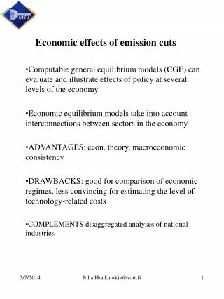
4. What is the VATTAGE? • Applied/Computable General Equilibrium Model for Finnish Economy • Bases on well-known ORANI and MONASH models http://www.monash.edu.au/policy/ • The model has been developed with the needs of several policy applications in mind • The model is intended as a tool for long term policy analysis • Model is ~fully documented and can be found from VATT’s homepage: http://www.vatt.fi/julkaisut/uusimmatJulkaisut/julkaisu/Publication_6093_id/832

5. Setting up the simulations • Baseline • National Accounts as starting point • Macroeconomic forecasts • AWG (the Ageing Working Group of European Council): long term projections for macro variables • Stability and growth pact • Industry specific forecasts • TEM; exports, transports, housing, construction, energy production, etc. • STAKES&VATT, AWG; Public services • Private consumption from model

6. Setting up the simulations • Policies 1) EU committed to Kyoto targets and emission trading • EU has set target for 2020 emissions • -20% if go-it-alone • -30% if global 2) During the Kyoto period. Prices of emission permits rise to 25€/tCO2 by 2012, and to 30-45€/tCO2 by 2020 3) Policies for renewables • Feed-in tariffs for wind power and biogas • Tax cuts or subsidies for wood • Blending requirements for biofuels (10% by 2020) 4) Energy-saving measures in all sectors Analyses of different policies combined with energy sector model can be found from VATT’s homepage: http://www.vatt.fi/julkaisut/uusimmatJulkaisut/julkaisu/Publication_6093_id/796

7. Cumulative changes in GDP from baseline

8. Income distribution module • Main idea: top-down disaggregation of income and consumption to eight different household types (mimicking top-down regional effects calculus in Monash-type state models) • Consumption: consumption function parameters estimated • Income structure by household type linked to generic VATTAGE income categories • Population: each age cohort divided into household types • Partly endogenous based on changes in labor markets • Partly exogenous based on age-structure (population growth and ageing based on Statistics Finland’s population projection 2007) Note: less data needed than in a full-fledged several-household model; core model intact

9. Income distribution module (1/ Household types (Socio-economic Groups, classification code in brackets) • Farmer (10) • Entrepreneur (20) • Upper white-collar employee (30) • Lower white-collar employee (40) • Manual worker (50) • Student (60) • Retired (70) • Unemployed and others (80 + 90)

10. Income categories • Capital and land income • Labor income • Old-age benefits • Unemployment benefits • Other transfers

11. Data used in income distribution module • Income distribution statistics: Shares of different income types and tax rates from household income (~28,000 obs.) • Household Budget Survey 2006: expenditure shares by household type – estimation of consumption functions (4,007 obs.) • Fitted to aggregate household consumption data of VATTAGE (from national accounts) • Re-estimation of consumption function of the representative consumer

12. Cumulative changes in main Macroeconomic variables(full energy package – allowance price 30 €)

13. Contributions of GDP expenditure items to cumulative change(full energy package – allowance price 30 €)

14. Changes in industry structure(full energy package – allowance price 30 €) • Energy package changes industry output significantly • Decline in all industries except agriculture and forestry

15. Changes in industry structure(full energy package – allowance price 30 €) • Employment changes reflect changes in output

16. Aggregated household consumption in the VATTAGE model Estimated from Household budget survey Used estimates made in Global Trade Analysis Project (GTAP)

17. Share of energy of production costs by product (without energy products, <70%)

18. Consumption share of energy use in year 2005, per cent (both direct and indirect use included)

19. Change in income and real consumption in year 2020 by socio-economic group(per cent from base scenario, ordered by income level)

20. Contributions of product groups to changes in consumption volumes in 2020

21. What if we group households into income deciles? • Households divided into deciles by income / modified OECD consumption unit (but with equal population shares) • Another module with same data sources and with similar equations • The consumpion data would not allow creating soc.econ*decile = 80 groups into the core model

22. Consumption share of energy use in year 2005, per cent by decile(both direct and indirect use included)

23. Change in income and real consumption in year 2020 by income decile (per cent from base scenario)

24. Cumulative deviation from BASE in real consumption by income decile

25. Conclusions • Climate policy does not seem to be regressive in the light of our results: the large share income transfers among low-income earners decreases the negative income effect of climate policy • Farmers and low-income earners winners in relation to other households when effects are measured through changes in consumption volume – income measures tell a different story • Indirect use of energy evens out the effects of climate policy; analysis concentrating in consumption of energy products and (directly) energy-intensive products leads to wrong conclusions about the distributional effects • The direction of conclusions hinges on the effects stemming from consumption patterns – consumption elasticity parameters are important • Results with other consumption functions than LES? - Actually, changing the consumption functions into Cobb-Douglas does not change the qualitative story at all, and even numbers change only a little -> what seems to matter is differences in the consumption shares