Download
1 / 56
570 likes | 749 Views
Unsupervised Learning. G.Anuradha. Contents. Introduction Competitive Learning networks Kohenen self-organizing networks Learning vector quantization Hebbian learning. Introduction.

E N D
Unsupervised Learning G.Anuradha
Contents • Introduction • Competitive Learning networks • Kohenen self-organizing networks • Learning vector quantization • Hebbian learning
Introduction The main property of a neural network is an ability to learn from its environment, and to improve its performance through learning. So far we have considered supervised or active learning- learning with an external “teacher” or a supervisor who presents a training set to the network. But another type of learning also exists: unsupervised learning.
In contrast to supervised learning, unsupervised or self-organised learning does not require an external teacher. During the training session, the neural network receives a number of different input patterns, discovers significant features in these patterns and learns how to classify input data into appropriate categories. Unsupervised learning tends to follow the neuro-biological organisation of the brain. • Unsupervised learning algorithms aim to learnrapidly and can be used in real-time.
Hebbian learning In 1949, Donald Hebb proposed one of the key ideas in biological learning, commonly known as Hebb’s Law. Hebb’s Law states that if neuron iis near enough to excite neuron j and repeatedly participates in its activation, the synaptic connection between these two neurons is strengthened and neuron j becomes more sensitive to stimuli from neuron i.
Hebb’s Law can be represented in the form of two rules: • If two neurons on either side of a connection are activated synchronously, then the weight of that connection is increased. • If two neurons on either side of a connection are activated asynchronously, then the weight of that connection is decreased. • Hebb’s Law provides the basis for learning without a teacher. Learning here is a local phenomenon occurring without feedback from the environment.
Competitive learning • In competitive learning, neurons compete among themselves to be activated. • While in Hebbian learning, several output neurons can be activated simultaneously, in competitive learning, only a single output neuron is active at any time. • The output neuron that wins the “competition” is called the winner-takes-all neuron.
The basic idea of competitive learning was introduced in the early 1970s. • In the late 1980s, TeuvoKohonen introduced a special class of artificial neural networks called self-organizing feature maps. These maps are based on competitive learning. Intelligent Systems and Soft Computing
What is a self-organizing feature map? Our brain is dominated by the cerebral cortex, a very complex structure of billions of neurons and hundreds of billions of synapses. The cortex includes areas that are responsible for different human activities (motor, visual, auditory, somatosensory, etc.), andassociated with different sensory inputs. We can say that each sensory input is mapped into a corresponding area of the cerebral cortex. The cortex is a self-organizing computational map in the human brain. Intelligent Systems and Soft Computing
Kohenen Self-Organizing Feature Maps • Feature mapping converts a wide pattern space into a typical feature space • Apart from reducing higher dimensionality it has to preserve the neighborhood relations of input patterns
Feature-mapping Kohonen model Intelligent Systems and Soft Computing
The Kohonen network • The Kohonen model provides a topological mapping. It places a fixed number of input patterns from the input layer into a higher- dimensional output or Kohonen layer. • Training in the Kohonen network begins with the winner’s neighborhood of a fairly large size. Then, as training proceeds, the neighborhood size gradually decreases.
Model: Horizontal & Vertical linesRumelhart & Zipser, 1985 • Problem – identify vertical or horizontal signals • Inputs are 6 x 6 arrays • Intermediate layer with 8 units • Output layer with 2 units • Cannot work with one layer
H V Rumelhart & Zipser, Cntd
Geometrical Interpretation • So far the ordering of the output units themselves was not necessarily informative • The location of the winning unit can give us information regarding similarities in the data • We are looking for an input output mapping that conserves the topologic properties of the inputs feature mapping • Given any two spaces, it is not guaranteed that such a mapping exits!
In theKohonen network, a neuron learns by shifting its weights from inactive connections to active ones. Only the winning neuron and its neighbourhood are allowed to learn. If a neuron does not respond to a given input pattern, then learning cannot occur in that particular neuron. • The competitive learning rule defines the change Dwijapplied to synaptic weight wijas where xiis the input signal and ais the learning rate parameter. Intelligent Systems and Soft Computing
The overall effect of the competitive learning rule resides in moving the synaptic weight vector Wjof the winning neuron j towards the input pattern X. The matching criterion is equivalent to the minimum Euclidean distance between vectors. • The Euclidean distance between a pair of n-by-1 vectors X and Wjis defined by where xiand wijare the ith elements of the vectors X and Wj, respectively. Intelligent Systems and Soft Computing
To identify the winningneuron, jX, that best matches the input vector X, we may apply the following condition: • where m is the number of neurons in the Kohonen layer. Intelligent Systems and Soft Computing
Suppose, for instance, that the 2-dimensional input vector X is presented to the three-neuron Kohonen network, • The initial weight vectors, Wj, are given by Intelligent Systems and Soft Computing
We find the winning (best-matching) neuron jXusing the minimum-distance Euclidean criterion: • Neuron 3 is the winner and its weight vector W3 is updated according to the competitive learning rule. Intelligent Systems and Soft Computing
The updated weight vector W3 at iteration (p + 1) is determined as: • The weight vector W3 of the wining neuron 3 becomes closer to the input vector X with each iteration. Intelligent Systems and Soft Computing
Measures of similarity Distance Normalized scalar product
Also known as Kohenen Feature maps or topology-preserving maps • Learning procedure of Kohenen feature maps is similar to that of competitive learning networks. • Similarity (dissimilarity) measure is selected and the winning unit is considered to be the one with the largest (smallest) activation • The weights of the winning neuron as well as the neighborhood around the winning units are adjusted. • Neighborhood size decreases slowly with every iteration.
Training of kohenon self organizing network • Select the winning output unit as the one with the largest similarity measure between all wi and xi . The winning unit c satisfies the equation ||x-wc||=min||x-wi|| where the index c refers to the winning unit (Euclidean distance) • Let NBc denote a set of index corresponding to a neighborhood around winner c. The weights of the winner and it neighboring units are updated by Δwi=ɳ(x-wi) iεNBc
For Each i/p X Initialize Weights, Learning rate Initialize Topological Neighborhood params Start For i=1 to n For j=1 to m D(j)=Ʃ(xi-wij)2 Winning unit index J is computed D(J)=minimum Weights of winning unit continue continue Stop Test (t+1) Is reduced Reduce radius Of network Reduce learning rate
Problem • Construct a kohenen self-organizing map to cluster the four given vectors [0 0 1 1], [1 0 0 0], [0 1 1 0],[0 0 01]. The number of cluster to be formed is two. Initial learning rate is 0.5 • Initial weights =
W(2,j) W(1,j) Network after 100 iterations Intelligent Systems and Soft Computing
W(2,j) W(1,j) Network after 1000 iterations Intelligent Systems and Soft Computing
W(2,j) W(1,j) Network after 10,000 iterations Intelligent Systems and Soft Computing
Training occurs in several steps and over many iterations: Each node's weights are initialized. A vector is chosen at random from the set of training data and presented to the lattice. Every node is examined to calculate which one's weights are most like the input vector. The winning node is commonly known as the Best Matching Unit (BMU). The radius of the neighbourhood of the BMU is now calculated. This is a value that starts large, typically set to the 'radius' of the lattice, but diminishes each time-step. Any nodes found within this radius are deemed to be inside the BMU's neighbourhood. Each neighbouring node's (the nodes found in step 4) weights are adjusted to make them more like the input vector. The closer a node is to the BMU, the more its weights get altered. Repeat step 2 for N iterations.
A neighborhood function around the winning unit can be used instead of defining the neighborhood of a winning unit. • A Gaussian function can be used as neighborhood function Where pi and pc are the positions of the output units i and c respectively and σ reflects the scope of the neighborhood. The update formula using neighborhood function is given by
What happens in a dot product method? • In the case of a dot product finding a minimum of x-wi is nothing but finding the maximum among the m scalar products
Competitive learning network performs an on-line clustering process on the input patterns • When process is complete the input data is divided into disjoint clusters • With euclidean distance the update formula is actually an online gradient descent that minimizes the objective function
Competitive learning with unit-length vectors The dots represent the input vectors and the crosses denote the weight vectors for the four output units As the learning continues, the four weight vectors rotate toward the centers of the four input clusters
Limitations of competitive learning • Weights are initialized to random values which might be far from any input vector and it never gets updated • Can be prevented by initializing the weights to samples from the input data itself, thereby ensuring that all weights get updated when all the input patterns are presented • Or else the weights of winning as well as losing neurons can be updated by tuning the learning constant by using a significantly smaller learning rate for the losers. This is called as leaky learning • Note:- Changing η is generally desired. An initial value of η explores the data space widely. Later on progressively smaller value refines the weights. Similar to the cooling schedule in simulated annealing.
Limitations of competitive learning • Lacks the capability to add new clusters when deemed necessary • If ɳ is constant –no stability of clusters • If ɳ is decreasing with time may become too small to update cluster centers • This is called as stability-plasticity dilemma (Solved using adaptive resonance theory (ART))
If the output units are arranged in the form of a vector or matrix then the weights of winners as well as neighbouring losers can be updated. (Kohenen feature maps) • After learning the input space is divided into a number of disjoint clusters. These cluster centers are known as template or code book • For any input pattern presented we can use an appropriate code book vector (Vector Quantization) • This vector quantization is used in data compression in IP and communication systems.
LVQ • Recall that a Kohonen SOM is a clustering technique, which can be used to provide insight into the nature of data. We can transform this unsupervised neural network into a supervised LVQ neural network. • The network architecture is just like a SOM, but without a topological structure. • Each output neuron represents a known category (e.g. apple, pear, orange). • Input vector = x=(x1,x2…..xn) • Weight vector for the jth output neuron wj=( w1j,w2j,….wnj) • Cj= Category represented by the jth neuron. This is pre-assigned. • T = Correct category for input • Define Euclidean distance between the input vector and the weight vector of the jth neuron as:Ʃ(xi-wij)2
It is an adaptive data classification method based on training data with desired class information • It is actually a supervised training method but employs unsupervised data-clustering techniques to preprocess the data set and obtain cluster centers • Resembles a competitive learning network except that each output unit is associated with a class.