Download
1 / 29
300 likes | 393 Views
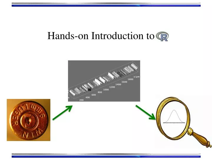
Hands-on Introduction to R. Outline. R : A powerful Platform for Statistical Analysis Why bother learning R ? Data, data, data, I cannot make bricks without clay Copper Beeches A tour of RStudio . Basic Input and Output Getting Help Loading your data from Excel spreadsheets

E N D
Outline • R : A powerful Platform for Statistical Analysis • Why bother learning R ? • Data, data, data, I cannot make bricks without clay Copper Beeches • A tour of RStudio. Basic Input and Output • Getting Help • Loading your data from Excel spreadsheets • Visualizing with Plots • Basic Statistical Inference Tools • Confidence Intervals • Hypothesis Testing/ANOVA
Why ? • R is not a black box! • Codes available for review; totally transparent! • R maintained by a professional group of statisticians, and computational scientists • From very simple to state-of-the-art procedures available • Very good graphics for exhibits and papers • R is extensible (it is a full scripting language) • Coding/syntax similar to Python and MATLAB • Easy to link to C/C++ routines
Why ? • Where to get information on R : • R: http://www.r-project.org/ • Just need the base • RStudio: http://rstudio.org/ • A great IDE for R • Work on all platforms • Sometimes slows down performance… • CRAN: http://cran.r-project.org/ • Library repository for R • Click on Search on the left of the website to search for package/info on packages
Finding our way around R/RStudio Script Window Command Line
Handy Commands: • Basic Input and Output Numeric input x <- 4 variables: store information :Assignment operator x <- “text goes in quotes” Text (character) input
Handy Commands: • Get help on an R command: • If you know the name: ?command name • ?plot brings up html on plot command • If you don’t know the name: • Use Google (my favorite) • ??key word
Handy Commands: • R is driven by functions: func(arguement1, argument2) input to function goes in parenthesis function name function returns something; gets dumped into x x <- func(arg1, arg2)
Handy Commands: • Input from Excel • Save spreadsheet as a CSV file • Use read.csv function • Needs the path to the file Mac e.g.: "/Users/npetraco/latex/papers/data.csv” Windows e.g.: “C:\Users\npetraco\latex\papers\data.csv” *Exercise: basicIO.R
Handy Commands: • Matrices: X • X[,1] returns column 1 of matrix X • X[3,] returns row 3 of matrix X • Handy functions for data frames and matrices: • dim, nrow, ncol, rbind, cbind • User defined functions syntax: • func.name <- function(arguements) { • do something • return(output) • } • To use it: func.name(values)
First Thing: Look at your Data • Explore the Glass dataset of the mlbench package • Source (load) all_data_source.R • *visualize_with_plots.r • Scatter plots: plot any two variables against each other
First Thing: Look at your Data • Pairs plots: do many scatter plots at once
First Thing: Look at your Data • Histograms: “bin” a variable and plot frequencies
First Thing: Look at your Data • Histograms conditioned on other variables: use lattice package RIs Conditioned on glass group membership
First Thing: Look at your Data • Probability density plots: also needs lattice
First Thing: Look at your Data • Empirical Probability Distribution plots: also called empirical cumulative density
First Thing: Look at your Data • Box and Whiskers plots: range possible outliers possible outliers 25th-%tile 1st-quartile 75th-%tile 3rd-quartile median 50th-%tile RI
Visualizing Data • Note the relationship:
First Thing: Look at your Data • Box and Whiskers plots: Box-Whiskers plots for actual variable values Box-Whiskers plots for scaled variable values
Confidence Intervals • A confidence interval (CI) gives a range in which a true population parameter may be found. • Specifically,(1-)×100% CIs for a parameter, constructed from a random sample (of a given sample size), will contain the true value of the parameter approximately (1-)×100% of the time. • Different from tolerance and prediction intervals
Confidence Intervals • Caution: IT IS NOT CORRECT to say that there a (1-)×100% probability that the true valueof a parameter is between the bounds of any given CI. Take a sample. Compute a CI. Here 90% of the CIs contain the true value of the parameter Graphical representation of 90% CIs is for a parameter: true value of parameter
Confidence Intervals • Construction of a CI for a mean depends on: • Sample size n • Standard error for means • Level of confidence 1- • is significance level • Use to compute tc-value • (1-)×100% CI for population mean using a sample average and standard error is:
Confidence Intervals • Compute a 99% confidence interval for the mean using this sample set: (/2=0.005) tc = 3.17 Putting this together: [1.52005 - (3.17)(0.00001), 1.52005 + (3.17)(0.00001)] 99% CI for sample = [1.52002, 1.52009] *Try out confidence_intervals.R
Hypothesis Testing • A hypothesis is an assumption about a statistic. • Form a hypothesis about the statistic • H0, the null hypothesis • Identify the alternative hypothesis, Ha • “Accept” H0 or “Reject” H0 in favour of Ha at a certain confidence level (1-)×100% • Technically, “Accept” means “Do not Reject” • The testing is done with respect to how sample values of the statistic are distributed • Student’s-t • Gaussian • Binomial • Poisson • Bootstrap, etc.
Hypothesis Testing • Hypothesis testing can go wrong: • 1- is called test’s power • Do the thicknesses of float glass differ from non float glass? • How can we use a computer to decide?
Analysis of Variance • Standard hypothesis testing is great for comparing two statistics. • What is we have more than two statistics to compare? • Use analysis of variance (ANOVA) • Note that the statistics to be compares must all be of the same type • Usually the statistic is an average “response” for different experimental conditions or treatments.
Analysis of Variance • H0 for ANOVA • The values being compared are not statistically different at the (1-)×100% level of confidence • Ha for ANOVA • At least one of the values being compared is statically distinct. • ANOVA computes an F-statistic from the data and compares to a critical Fc value for • Level of confidence • D.O.F. 1 = # of levels -1 • D.O.F. 2 = # of obs. - # of levels
Analysis of Variance • H0 for ANOVA • The values being compared are not statistically different at the (1-)×100% level of confidence • Ha for ANOVA • At least one of the values being compared is statically distinct. • ANOVA computes an F-statistic from the data and compares to a critical Fc value for • Level of confidence • D.O.F. 1 = # of levels -1 • D.O.F. 2 = # of obs. - # of levels
Analysis of Variance • Levels are “categorical variables” and can be: • Group names • Experimental conditions • Experimental treatments • Are the average RIs for each type of glass in the “Forensic Glass” data set statistically different? Exercise: Try out anova.R