Download
1 / 58
610 likes | 801 Views
Value at Risk Modelling for Energy Commodities using Volatility Adjusted Quantile Regression. Energy Finance Conference Essen Thursday 10 th October 2013 Sjur Westgaard Email: sjur.westgaard@iot.ntnu.no Tel: 73593183 / 91897096 Web: www.iot.ntnu.no/users/sjurw

E N D
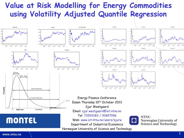
Value at Risk Modelling for Energy Commodities using Volatility Adjusted Quantile Regression Energy Finance Conference Essen Thursday 10th October 2013 Sjur Westgaard Email: sjur.westgaard@iot.ntnu.no Tel: 73593183 / 91897096 Web: www.iot.ntnu.no/users/sjurw Department of Industrial Economics Norwegian University of Science and Technology
Professor Sjur Westgaard Department of Industrial Economics and Technology Management, Norwegian University of Science and Technology (NTNU) Alfred Getz vei 3, NO-7491 Trondheim, Norway www.ntnu.no/iot Mail: sjur.westgaard@iot.ntnu.no Web: www.iot.ntnu.no/users/sjurw Phone: +47 73598183 or +47 91897096 Sjur Westgaard is MSc and Phd in Industrial Economics from Norwegian University of Science and Technology and a MSc in Finance from Norwegian School of Business and Economics. He has worked as an investment portfolio manager for an insurance company, a project risk manager for a consultant company and as a credit analyst for an international bank. His is now a Professor at the Norwegian University of Science and Technology and an Adjunct Professor at the Norwegian Center of Commodity Market Analysis UMB Business School. His teaching involves corporate finance, derivatives and real options, empirical finance and commodity markets. His main research interests is within risk modelling of energy markets and he has been a project manager for two energy energy research projects involving power companies and the Norwegian Research Consil. He has also an own consultancy company running executive courses and software implementations for energy companies. Part of this work is done jointly with Montel.
Trondheim Trondheim
Montel Online • Up-to-the-minute news • Live price feeds European Energy Data • Price-driving fundamentals • Financial / weather data • Excel-addin historical data • Courses and Seminars
Why Value at Risk Modelling for Energy Commodities using Volatility Adjusted Quantile Regression? • From Burger et al. (2008)*: • Liberalisation of energy markets (oil, gas, coal, el, carbon) has fundamentally changed the way power companies do business • Competition has created both strong incentives for improving operational efficiency and as well as the need for effective financial risk management * Burger, M., Graeber B., Schindlmayr, G. 2008, Managing energy risk – An integrated view on power and other energy markets, Wiley. 6
Why Value at Risk Modelling for Energy Commodities using Volatility Adjusted Quantile Regression? • More volatile energy markets and complex trading/hedging portfolios (long and short positions) has increased the need for measuring risk at • Individual contract level • Portfolio of contracts level • Enterprise level • Understanding the dynamics and determinants of volatility and risk (e.g. Value at Risk and Expected Shortfall) for energy commodities are therefore crucial. • We therefore need to correctly model and forecast the return distribution for energy futures markets 7
Why Value at Risk Modelling for Energy Commodities using Volatility Adjusted Quantile Regression? • Oil/GasOil/Natural Gas/Coal/Carbon/Electricity from ICE, EEX, Nasdaq OMX shows: • Conditional return distributions various across energy commodities • Conditional return distributions for energy commodities varies over time • This makes risk modelling of energy futures markets very challenging!
The problems with existing “standard” risk model (that many energy companies have adopted from the bank industry) are: • RiskmetricsTMVaRcapture time varying volatility but not the conditional return distribution • Historical Simulation VaRcapture the return distribution but not the time varying volatility • Alternatives: • GARCH with T, Skew T, or GED • CaViaR type models • Although these models works fine according to several studies, there is a problem of calibrating these non-linear models and therefore they are only used to a very limited extent in practice Why Value at Risk Modelling for Energy Commodities using Volatility Adjusted Quantile Regression?
In this paper we propose a robust and “easy to implement” approach for Value at Risk estimation based on; • First running an exponential weighted moving average volatilitymodel (similar to the adjustment done in RiskmetricsTM) and then • Run a linear quantile regression model based on this conditional volatility as input/explanatory variable • The model is easy to implement (can be done in a spreadsheet) • This model also shows an excellent fit when backtestingVaR Why Value at Risk Modelling for Energy Commodities using Volatility Adjusted Quantile Regression?
Measuring Value at Risk / Quantiles Loss for a consumer or trader having a short position in German front Quarter Futures. Loss for a producer or trader having a long position in German front Quarter Futures. One important task is to model and forecast the upper and lower tail of the price distribution using standard risk measures such as Value at Risk and Conditional Value at Risk for different quantiles (e.g. 0.1%, 1%, 5%, 10%, 90%, 95%, 99%, 99.9%). Oil prices ($/Ton)
Previous work/literature of risk modelling of (energy) commodities • European Energy Futures Markets (crude oil, gas oil, natural gas, coal, carbon, and electricity) and Data/Descriptive Statistics • ICE • ICE-ENDEX • EEX • Nasdaq OMX Commodities • Volatility Adjusted Quantile Regression • Comparing / Backtesting Value at Risk analysis for Energy Commodities • RiskMetricsTM • Historical Simulation • Volatility Adjusted Quantile Regression • Conclusions and further work Layout for the presentation
Literature • Value at Risk analysis for energy and other commodities:: • Andriosopoulos and Nomikos (2011) • Aloui (2008) • Borger et al (2007) • Bunn et al. (2013) • Chan and Gray (2006) • Cabedo and Moya (2003) • Costello et al. (2008) • Fuss et al. (2010) • Giot and Laurent (2003) • Hung et al. (2008) • Mabrouk (2011) • Quantile regression in general and applications in financial risk management: • Alexander (2008) • Engle and Manganelli (2004) • Hao and Naiman (2007) • Koenker and Hallock (2001) • Koenker (2005) • Taylor (2000, 2008a, 2008b,2011) We want to fill the gap in the literature by performing Value at Risk analysis for European Energy Futures using volatility adjusted quantile regression. • Discussion weaknesses RiskMetrics and Historical Simulation during Financial Crises • Sheedy (2008a, 2008b)
Literature TEXTBOOKS ENERGY MARKET MODELLING • Bunn D., 2004, Modelling Prices in Competitive Electricity Markets , Wiley • Burger, M., Graeber B., Schindlmayr, G. 2008, Managing energy risk – An integrated view on power and other energy markets, Wiley. • Eydeland A. and Wolyniec K., 2003, Energy and power risk management, Wiley • Geman H., 2005, Commoditites and commodity derivatives – Modelling and pricing for agriculturas, metals and energy, Wiley • Geman H., 2008, Risk Management in commodity markets – From shipping to agriculturas and energy, Wiley • Kaminski V., 2005,Managing Energy Price Risk – The New Challenges and Solutions, Risk Books • Kaminski V., 2005,Energy Modelling, Risk Books • Kaminski V., 2013,Energy Morkets, Risk Books • Pilipovic D., 2007, Energy risk – Valuation and managing energy derivatives, McGrawHill • Serletis A., 2007. Quantitative and empirical analysis of energy markets, Word Scientific • Weron R., 2006, Modeling and Forecasting Electricity Loads and Prices: A Statistical Approach, Wiley
European Energy Futures and Options Markets ICE: www.theice.com ICE-ENDEX: www.iceendex.com EEX: www.eex.com Nasdaq OMX commodities: www.nasdaqcommodities.com
Data and descriptive statisticsPhase II Dec 2013 Futures Contract
Data and descriptivestatisticsUK Base Front Month and Quarter Futures Contracts
Data and descriptivestatisticsDutch Base Front Month and Quarter Futures Contracts
Data and descriptivestatisticsGerman Base Front Month and Quarter Futures Contracts
Data and descriptivestatistics Nordic Base Front Month and Quarter Futures Contracts
Data and descriptive statistics • Returns are calculated as relative price changes ln(Pt/Pt-1) for crude oil, gas oil, natural gas, coal, carbon, month and quarter base contracts for UK, Nederland, Germany, and the Nordic market • Returns when contract rolls over are deleted
Data and descriptive statistics • Mean, Stdev, Skew, Kurt, Min, Max, Empirical 5% and 95% quantiles are estimated for all series in the following periods: • 13Oct2008 to 30Dec2008 • 2009 • 2010 • 2011 • 2012 • 02Jan2013 to 30Sep2013 • 13Oct2008 to 30Sep2013 • Questions in mind: • How do return distributions varies across energy commodities? • How do energy commodity distributions changes over time?
Data and descriptive statistics Example of analysis: German and Nordic Rolling Base Front Quarter Contracts
Data and descriptive statistics • High return volatility for energy commodities. Annualized values much higher than for stocks and currency markets, specially for short term natural gas and electricity contracts • Fat tails for all energy commodities. Some energy commodities have mainly negative skewness (e.g. crude oil), others positive (e.g natural gas) • Return distribution of energy commodities varies a lot over time, hence the evolution of empirical VaR over time • Risk modeling of energy commodities will be very challenging. Need models that capture the dynamics of changing return distribution over time
Quantile regression • Quantile regression was introduced by a paper in Econometrica with Koenker and Bassett (1978) and is fully described in books by Koenker (2005) and Hao and Naiman (2007) • Applications in financial risk management (stocks / currency markets) can be found by Engle and Manganelli (2004), Alexander (2008), Taylor (2008) 28
Quantile regression 0.1, 0.5, and 0.9 quantile regression lines. The lines are found by the following minimizing the weighted absolute distance to the qth regression line: Yqt = αq+βqXt+εqt 29
Volatility Adjusted Quantile Regression 1) Calculate Exponentially Weighted Moving Average of Volatility 2) Run a Quantile Regression Regression with the Exponentially Weighted Moving Average of Volatility as the explanatory variable 3) Predict the VaRqt+1 from the model
Returns and EWMA Volatility Example El_Ger_Q This is just an Excel illustration. Qreg procedures in R, Stata, Eviews etc. should be used instead 31
Returns and EWMA Volatility Example GasOil
Returns and EWMA Volatility Example GasOil Distribution forecast from volatility adjusted quantile regression Todays EWMA vol is 2% on a daily basis. What is 5%, 95% 1 day VaR given our model? Var5% = -0.006589 % - 1.290804*2% = -2.59% Var5% = -0.002108 % + 1.817529 *2% = 3.63% Similar equations are found for all the quantiles
Comparing Value at Risk models for energy commodities • VaR Models • RiskMetricsTM • Historical Simulation • Volatility Adjusted Quantile Regression • Backtesting Value at Risk Models • Kupiec Test • Christoffersen Test
Comparing Value at Risk models for energy commodities • It is easy to estimate VaR once we have the return distribution • The only difference between the VaR models are due to the manner in which this distribution is constructed
Comparing Value at Risk models for energy commodities • RiskMetricsTM • Analytically tractable, adjustment for time-varying volatility, but assumption of normally distributed returns for energy commodities is not suitable
RiskMetricsTM VaRα=Ф-1(α)*σt Volatility changes dynamically over time and needs to be updated. For this reason many institutions use an exponentially weighted moving average (EWMA) methodology for VaR estimation, e.g. using EWMA to estimate volatility in the normal linear VaR formula These estimates take account of volatility clustering so that EWMA VaR estimates are more risk sensitive
Comparing Value at Risk models for energy commodities • Historical simulation • Makes no assumptions about the parametric form of the return distribution, but do not make the distribution conditional upon market conditions / volatility
Historical Simulation • Choose a sample size to reflect current market conditions (Banks usually use 3-5 years) • Draw returns from the empirical distribution and calculate VaR for each simulation • Use the average VaR for all simulation (you alsp get the distribution of VaR as an outcome) • Also called bootstrapping
Comparing Value at Risk models for energy commodities • Volatility Adjusted Quantile Regression • Allows for all kinds of distributions (semi non-parametric method) and allow the distribution to be conditional upon the volatility/changing market condition
Volatility Adjusted Quantile Regression 1) Calculate Exponentially Weighted Moving Average of Volatility 2) Run a Quantile Regression Regression with the Exponentially Weighted Moving Average of Volatility as the explanatory variable 3) Predict the VaRqt+1 from the model
Backtesting VaR Models In sample analysis • Backtesting refers to testing the accuracy of a VaR model over a historical period when the true outcome (return) is known • The general approach to backtesting VaR for an asset is to record the number of occasions over the period when the actual loss exceeds the model predicted VaR and compare this number to the pre-specified VaR level
Backtesting VaR Models Example Front Quarter Futures Nordic
Backtesting Value at Risk Models • A proper VaR model has: • The number of exceedances as close as possible to the number implied by the VaR quantile we are trying to model • Exceedances that are randomly distributed over the sample (that is no “clustering” of exceedances). We do not want the model to over/under predict VaR in certain periods
Backtesting VaR Models • To validate the predictive performance of the models, we consider two types of test: • The unconditional test of Kupiec (1995) • The conditional coverage test of Christoffersen (1998) • Kupiec (1995) test whether the number of exceedances or hits are equal to the predefined VaR level. Christoffersen (1998) also test whether the exceedances/hits are randomly distributed over the sample
Backtesting Value at Risk Models – Kupiec Test The Kupiec (1995) test is a likelihood ratio test designed to reveal whether the model provides the correct unconditional coverage. More precisely, let Ht be a indicator sequence where Ht takes the value 1 if the observed return, Yt, is below the predicted VaR quantile, Qt, at time t
Backtesting Value at Risk Models – Kupiec Test Under the null hypothesis of correct unconditional coverage the test statistic is Where n1 and n0 is the number of violations and non-violations respectively, πexp is the expected proportion of exceedances and πobs = n1/(n0+n1) the observed proportion of exceedances.