Download

1 / 10
100 likes | 267 Views
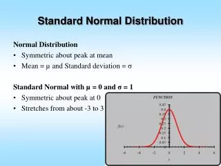
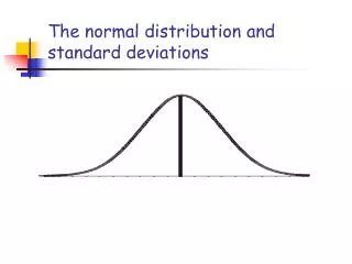
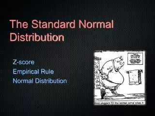
The Standard Normal Distribution. Standard Normal Density Curve. The standard normal distribution has a mean = 0 and a standard deviation = 1 Values on the x-axis are the number of standard deviations from the mean, called z-scores Interactive Applet: www.whfreeman.com/sta

E N D
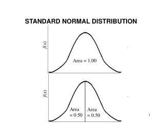
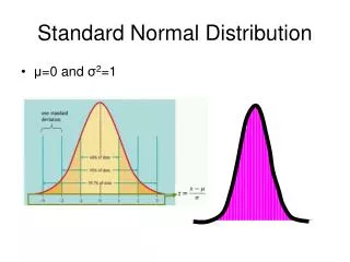
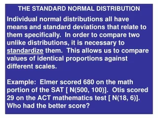
Standard Normal Density Curve • The standard normal distribution has a mean = 0 and a standard deviation = 1 • Values on the x-axis are the number of standard deviations from the mean, called z-scores • Interactive Applet: www.whfreeman.com/sta • What percent of the observations lie within 1 standard deviation? • What if we wanted to know the percent of observations that lie within 1.5 standard deviations?
Using z-score table • The area to the left of the corresponding z- score is the percentage of observations, P, that fall below the z-score. • 1. Use the table to find the percentage of values below z = -1.2. • 11.51% • 2. What is P(z > -1.2)? • 100 – 11.51 = 88.49% • 3. What is P(-1.2 < z < 1.2)? • 88.49 – 11.51 = 76.98%
Using z-scores with a calculator • Use the normalcdf command to compute probabilities using the normal curve. • Press 2nd, DIST, normalcdf(lower boundary, upper boundary). Use -10 or 10 for ± infinity. • For example, to find P(z < 1) = normalcdf(-10, 1) • 1. Use the calculator to find the percentage of values below z = -1.2. • 2. What is P(z > -1.2)? • 3. What is P(-1.2 < z < 1.2)? Normalcdf(-10,-1.2)= .1151 = 11.51% Normalcdf(-1.2, 10)= .8849 = 88.49% Normalcdf(-1.2,1.2)= .7699 = 76.99%
(z- scores) Z = A positive z- score indicates the number of standard deviations above the mean A negative z- score indicates the number of standard deviations below the mean.
Using the normal curve to find percents • Find percent below (or the percentile of) a certain value • Use the formula to find the z-score and use table or use calculator: normalcdf with lower boundary of -10, upper is z • Find percent above a certain value • Use the formula to find the z-score and subtract table value from 100% or use calculator: normalcdf (lower boundary is z, upper is 10) • Find percent between two certain values • Use the formula to find two z-scores, one for each value • Use the table to find two percents and subtract them from each other ….or…. • Use calculator: normalcdf(lower is 1st z, upper is 2nd z)
SAT Example • The approximately normal distribution of SAT scores for the 2009 incoming class at the University of Texas had a mean 1815 and a standard deviation 252. • What is the z- score for a University of Texas student who got 1901 on the SAT? • Z = 1900 – 1815= 0.34 252 What percentage did better than this student? • P(z > .34) = Normalcdf(.34, 10) = .366 or 36.6% What percentile was a student at if he made a 2200? z = (2200-1815)/252 = 1.53 normalcdf(-10,1.53) = 94%
Heights Example • The heights of 18 to 24 year old males in the US are approximately normal with mean 70.1 inches and standard deviation 2.7 inches. The heights of 18 to 24 year old females have a mean of 64.8 inches and a standard deviation of 2.5 inches. • Estimate the percentage of US males between 18 and 24 who are 6ft tall or taller. • Z = 72 – 70.1= .7037 2.7 • P(z > .7037) = normalcdf(.7037, 10) = .2408 = 24.08% • Estimate the percentage of US females between 18 and 24 who are between 5 feet and 5’5”. • Z = 60 – 64.8 = -1.92 z = 65 – 64.8 = .08 2.5 2.5 P(-1.92 < z < .08) = normalcdf(-1.92,.08) = .5044 = 50.44%
Comparison Example • Your friend Mark scored a 43 on Mrs. Johnson's chemistry test. The mean score in her class was a 38 and the standard deviation was 4. Marshall scored a 67 on his AP Calculus test and the mean in that class was a 65, with a standard deviation of 7. Whose score was better, relative to their classes? • Mark: z = (43 – 38)/4 = 1.25 • P(z < 1.25) = normalcdf(-10, 1.25) = .894 = 89.4th percentile • Marshall: z = (67 – 65)/7 = .286 • P(z < .286) = normalcdf(-10, .286) = .613 = 61.3rd percentile • Mark did better because he was further above the mean than Marshall and was in the 89th percentile compared to Marshall who was only in the 61st percentile.
Born to Run… • A study of elite distance runners found a mean body weight of 139.1 pounds with a standard deviation of 10.6 pounds. Assuming the distribution of weights is approximately normal, make a sketch of the weight distribution. • What percent of runners would have a body weight between 107.3 and 149.7 lb? 84% • 16% of runners would have a body weight less than how many pounds? 128.5 pounds • What percent of runners would have a body weight less than 130 pounds? Z = (130-139.1)/10.6 = .858; normalcdf(-10, -.858) = 19.5% • What percent of runners would have a body weight greater than 160 pounds? Z = (160-139.1)/10.6 = 1.97; normalcdf(1.97,10) = 2.4% 107.3 117.9 128.5 139.1 149.7 160.3 170.9