Download
1 / 28
280 likes | 370 Views
Orbit of 39 Laetitia. p = 30 p = 60 b/a = 0.7 c/a = 0.5 P = 7 h .527 0 = 0.4. GAIA observations. (mag) with respect to first observation. The general idea We assume that the objects are triaxial ellipsoids.

E N D
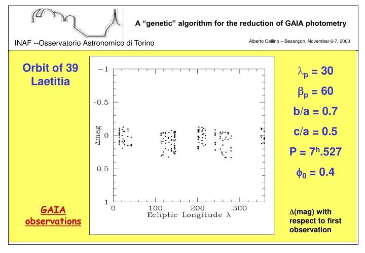
Orbit of 39 Laetitia • p = 30 p = 60 b/a = 0.7 c/a = 0.5 P = 7h.527 0 = 0.4 GAIA observations (mag) with respect to first observation
The general idea We assume that the objects are triaxial ellipsoids. We want to develop an automatic algorithm capable of finding a simultaneous solution for all the six parameters: Pole coordinates (P, P ) Sidereal Rotation Period (P) Axial ratios (b/a), (c/a) Rotational phase at epoch of first observation (0)
The purpose of determining the sidereal period implies that the use of pure computational “brute force” is not very recommendable, since the required accuracy for P is high: not smaller than 10-5 hours. This corresponds to an error in rotational phase of the order of 0.08 after five years of mission for P = 6 h. It follows that a very accurate solution using “brute force” would require alot of computing time. The number of iterations would be about: P b/a c/a P P 0
A different numerical approach has been chosen. We have developed an algorithm aimed at finding the overall solution of the problem (set of p, p, P, b/a, c/a, and 0 which produce the observed magnitudes), using atechnique of “genetic evolution” of the solutions. The idea is to make a much more efficient exploration of the space of the parameters, using an approach based on “the survival of the fittest”, similar to what happens in the biological world. According to the current state of the art, the code works fairly well, and requires a number of iterations less than 107, tipically.
In Paris (May 2003): Preliminary version of the algorithm Computations performed for zero-phase angle Simulations based on use of MBP observations
Now (November 2003): Improved algorithm Geometric effect of non 0-phase angle taken into account Assessment of the best detector to be used Simulations carried out accordingly
Geometric effect of non-zero phase This is taken into account using analytical solutions for the visible and illuminated portion of a triaxial ellipsoid asteroid with semiaxes a b c observed at a given phase angle 0, and at a given aspect and rotational phase. The formulas have been taken from published stuff (Pospieszalska-Surdej and Surdej, 1985) (after full checking and correction of a formula)
How it works 10,000 sets of parameters are randomly generated The “best” 1,000 sets are kept in an array The set of 1,000 best solutions starts to “genetically evolve”, by couple combination or random mutation of the parameters. At each generation, a check is made whether the newly born solution enters the Top 1,000 list. 1,500,000 iterations are performed. If no good solution is found, the procedure starts again from the beginning. A good solution is usually found !!
The goodness of each solution is estimated by means of the parameter: (other parameters could be used as well)
The “Genetic” algorithm At every step, one of the best 1,000 solutions is chosen. It generates a new “baby” solution either by finding a “mate” solution and exchanging randomly the respective parameters, or by duplicating itself, but with some random “mutation” of the parameters. A check is made that the new “baby” solution can enter the Top 1,000 list. The procedure is repeated for a maximum number of 1,500,000 steps, or until the parameter reaches a given value, corresponding to a good fit of the data.
(Old, i.e., May 2003) example of a bad solution > 0.05 Black boxes, “true” magnitudes (no error in the GAIA measurements, zero phase assumed)
(Old, i.e., May 2003) example of a good solution 0.001 mag Black boxes, “true” magnitudes (no error in the GAIA measurements, zero phase assumed)
A major improvement of the algorithm has been to introduce a tiny “transcription error” in the “DNA” of the solutions: Every time that one of the Top 1,000 solutions is randomly chosen for duplication during the “genetic” phase of the algorithm, a tiny error in the values of each of the six parameters is randomly introduced. This leads to a much quicker convergence of the resulting solution for the Sidereal Period to its “right” value (in the simulations)
Two numerical programs have been developed: A first program generates a set of simulated GAIA observations, being given a set of parameters, and a given nominal value for the error of the GAIA photometric measurements. A second program reads the simulated observations, and runs the genetic algorithm to find the right set of parameters. A third program is also used to generate randomly and blindly the “true” set of parameters for step 1.
In order to avoid that some systematic bug may affect both steps (1) and (2) of the simulations, some tests have also been done in which the “true” GAIA observations were numerically simulated by D. Hestroffer, using a completely independent numerical code. According to these tests, performed in August 2003, everything works correctly.
Photometric Errors of GAIA Detectors Asteroids are variable objects, then what is important for our purposes is the photometric accuracy of the different detectors for single observations (NOT for averages over five years of mission). According to current estimates, the photometric accuracy of the astrometric detector and of the MBP for a single measurement of an object are: Astrometric field: 0.01 mag for G 18.5 MBP (F63B) : 0.08 mag for V 19.0
Bad News The encouraging simulations shown in previous Paris meeting were based on the assumption of using the MBP. Using the astrometric fields detections, which have the kind of photometric accuracy we need, we have quite smaller numbers of available observations (for Laetitia, 70 against 200)
F.Mignard’s simulations id/name nobs prec foll spec mbp 1 Ceres 310 32 34 85 159 2 Pallas 292 28 26 70 168 3 Juno 274 29 33 69 143 4 Vesta 243 27 29 67120 5 Astraea 310 37 39 83 151 6 Hebe 206 23 20 54 109 7 Iris 319 33 30 75 181 8 Flora 266 29 29 69 139 9 Metis 236 22 26 63125 10 Hygiea 258 28 27 69 134 11 Parthenope 180 13 18 41 108 12 Victoria 240 28 26 62 124
Good News Even with a much smaller number of available observations, the “genetic” algorithm works fine. The algorithm works fine even when the assumed error on GAIA photometric measurements is assumed to be fairly large.
Again, we have used the results of the GAIA minor planet survey simulations carried out by F. Mignard. We have taken as a reference case the simulated GAIA detections of the asteroid 39 Laetitia (typical main-belt orbit). We have considered the detections in the GAIA astrometric field (about 70 observations). Different values for the nominal values of single observations have been considered (between 0.01 mag and 0.1 mag).
P between 2 and 24 hours b/a and c/a between 0.1 and 0.9, in different combinations (nearly-round to very elongated objects) P between 10o and 80o Both prograde and retrograde rotation Assumed photometric errors: 0.01, 0.02, 0.05, 0.1 mag Geometric effect of non-zero phase angle included The algorithm converges more or less quickly, but always it has been able so far to find the “right” solution (sometimes after N 10 runs). varies with error/3 as expected.
To be pessimistic, GAIA should photometrically measure with an accuracy of 0.01 mag in G, all the asteroids having H 12.5 (assuming V - H = 6, e Vlim = 18.5) The number of these objects is uncertain (not all of them have yet been discovered), but it should be of the order of 10,000 or slightly less. Taking into account that (a) GAIA can measure with 0.01 mag accuracy many objects fainter than H = 12.5, and (b) the genetic algorithm works well even when the photometric error is more than twice as large, we conclude that we should be able to find solutions (poles, Periods and axial ratios) for no less than 10,000 asteroids.
Things to do The major problem we have still to solve is to take into account the effect of light scattering. In the range between 10o and 30o, light scattering produces a fairly linear variation of magnitude with phase. This effect MUST be modelled.
Different options are possible: To derive independently the slope of the phase-magnitude relation from the observations, and to give this value in input to the genetic algorithm. To implement the determination of the magnitude-phase slope directly in the genetic algorithm, by adding it as a new free parameter. The next step of this analysis will be to check whether option (2) is feasible (adding a new parameter makes everything more difficult, in principle).
An obvious check of the effectiveness of the algorithm will be to apply it to the old HIPPARCOS data. This will be made when the effect of light scattering is properly taken into account. Preliminary tests using the current version of the algorithm have given unclear indications (in one case a reasonable solution has been found, in a few other cases the algorithm does not converge).
In terms of planning GAIA operations, it can be important to see whether it is possible to have in any case MBP observations of objects which are brighter than the saturation limit for the astrometric detectors. If this is possible, MBP could be used to measure bright objects, which will not be observed by the astrometric detectors, but for which the MBP photometric accuracy is good. These objects are important, since they are those for which we have most ground-based data, including estimates of Periods and Poles, to be used to check GAIA determinations.
The problem of the irregular shapes of real objects must also be taken into account, but the triaxial ellipsoid assumption is not expected to lead to major errors in many cases.