Download
1 / 23
250 likes | 401 Views
Solutions to the Advection-Dispersion Equation. Road Map to Solutions. We will discuss the following solutions Instantaneous injection in infinite and semi-infinite 1-dimensional columns Continuous injection into semi-infinite 1-D column

E N D
Road Map to Solutions • We will discuss the following solutions • Instantaneous injection in infinite and semi-infinite 1-dimensional columns • Continuous injection into semi-infinite 1-D column • Instantaneous point source solution in two-dimensions (line source in 3-D) • Instantaneous point source in 3-dimensions • Keep an eye on: • the initial assumptions • symmetry in space, asymmetry in time
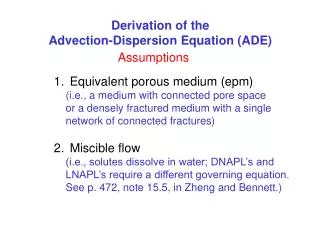
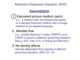
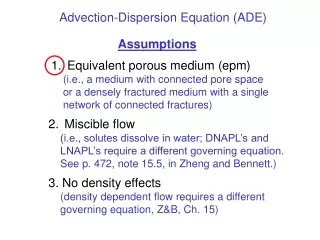
Recall the Governing Equation • What have we assumed thus far? • Dispersion can be expressed as a Fickian process • Diffusion and dispersion can be folded into a single hydrodynamic dispersion • First order decay • What do we need next? • More Assumptions!
Adding Sorption • Thus far we have addressed only the solute behavior in the liquid state. • We now add sorption using a linear isotherm • Recall the linear isotherm relationshipwhere cl and cs are in mass per volume of water and mass per mass of solid respectively • The total concentration is then
Retardation factor • We have • Which may be written as • where we have defined the retardation factor R to be
Putting this all together • The ADE with 1st order decay & linear isotherm • What do we need now? More assumptions! • constant in space (pull from derivatives + cancel) • D’ constant in space (slide it out of derivative) • R constant in time (slide it out of derivative) • Use the chain rule:the divergence of • a scalar =gradient;divergence of a constant is zero
Applying the previous assumptions • The divergence operators turn into gradient operators since they are applied to scalar quantities. • What does this give us? The new ADE
Looking at 1-D case for a moment • To see how this retardation factor works, take t* = t/R, and = 0. With a little algebra, • The punch line: • the spatial distribution of solutes is the same in the case of non-adsorbed vs. adsorbed compounds! • For a given boundary condition and time t*, the solution is unique and independent of R
1-D infinite column Instantaneous Point Injection velocity u • Column goes to +and - • Area A • steady velocity u • mass M injected at x = o and t=0(boundary condition) • initially uncontaminated column. i.e. c(x,0) = 0 (initial condition) • linear sorption (retardation R) • first order decay () x = 0
Features of solution: • Gaussian, symmetric in space, 2 = Dt/R • Exponential decay of pulse • Except for decay, R only shows up as t/R Upstream solutes Peak at 1.23 hr Center of Mass 2 hr Spatial Distribution Temporal Distribution
Putting this in terms of Pore Volumes • If solute transport is dominated by advection and dispersion, then the process is really only dependent on total water displacement (the two transport processes scale linerarly with time). • This would not be true if there were mass transfer between the mobile solution and liquid within the particles, or if diffusion were significant.
Pore Volume form of Solution Want concentration at x=L, in vs. pore-volumes passed through the system, P. Key substitutions: Coefficient n relates time and volume: nt=P At P=1, ut=L. This implies that u=Ln. This gives us: Now how do we get the n out?
Pore Volume Form of Solution • Note that D/n = DL/u = luL/u = lL • With this the result is entirely written in terms of the pore volumes and the media dispersivity, as we desired!
What about Retardation? • No Problem, just put it in as before:
1-D semi-infinite Instantaneous Point Injection • How do we handle a surface application? • Use the linearity of the simplified ADE • Can add any two solutions, and still a solution • By uniqueness, any solution which satisfies initial and boundary conditions is THE solution • Boundary and initial conditions
Semi-infinite solution • Upward pulse and downward. • Only include region of x > 0 in domain • Solution symmetric about x = 0, therefore slope of dc(x=0,t)/dx = 0 for all t, as required • Compared to infinite column, c starts twice as high, but in time goes to same solution
Continuous injection, 1-D • Since the simplified ADE is linear, we use superposition. Basically get a continuous injection solution by adding infinitely many infinitely small Gaussian plumes. • Use the complementary error function: erfc
Plot of solution • = 0.1, R = 1, = 0.02, u = 1.0, and m = 1
1-D, Cont., simplified • With no sorption or degradation this reduces to
2-D and 3-D instantaneous solutions Note: - Same Gaussian form as 1-D - Note separation of longitudinal and transverse dispersion
Review of Assumptions • Assumption Effects if Violated • constant in space -R higher where lower • -Velocity varies inversely with • D constant in space -Increased overall dispersion due • to heterogeneity • D independent of scale - Plume will grow more slowly at • first, then faster. • Reversible Sorption - Increase plume spreading and • overall region of contamination • Equilibrium Sorption - Increased “tailing” and spreading • Linear Sorption - Higher peak C and faster travel • Anisotropic media - Stretching & smearing along beds • Heterogeneous Media - Greater scale effects of D and ALL • EFFECTS DISCUSSED ABOVE