Integer Programming

1. Integer Programming • Introduction to Integer Programming (IP) • Difficulties of LP relaxation • IP Formulations • Branch and Bound Algorithms Reference: Chapter 9 in W. L. Winston’s book.

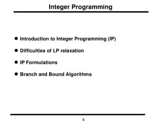
2. Integer Programming Model • An Integer Programming model is a linear programming problem where some or all of the variables are required to be non-negative integers. • These models are in general substantially harder than solving linear programming models. • Network models are special cases of integer programming models and are very efficiently solvable. • We will discuss several applications of integer programming models. • We will study the branch and bound technique, one of the most popular algorithm to solve integer programming models.

3. Classifications of IP Models Pure IP Model: Where all variables must take integer values. Maximize z = 3x1 + 2x2 subject to x1 + x2£ 6 x1, x2³ 0, x1 and x2 integer Mixed IP Model: Where some variables must be integer while others can take real values. Maximize z = 3x1 + 2x2 subject to x1 + x2£ 6 x1, x2³ 0, x1 integer 0-1 IP Model: Where all variables must take values 0 or 1 . Maximize z = x1 - x2 subject to x1 + 2x2£ 2 2x1 - x2£ 1, x1, x2 = 0 or 1

4. Classifications of IP Models (contd.) LP Relaxation: The LP obtained by omitting all integer or 0-1 constraints on variables is called the LP relaxation of IP. IP: Maximize z = 21x1 + 11x2 subject to 7x1 + 4x2£ 13 x1, x2³ 0, x1 and x2 integer LP Relaxation: Maximize z = 21x1 + 11x2 subject to 7x1 + 4x2£ 13 x1, x2³ 0 Result: Optimal objective function value of IP £ Optimal obj. function value of LP relaxation

5. x x x x IP and LP Relaxation 3 2 7x1 + 4x2= 13 x2 1 x x x x 3 1 2 x1

6. Simple Approaches for Solving IP Approach 1: • Enumerate all possible solutions • Determine their objective function values • Select the solution with the maximum (or, minimum) value. Any potential difficulty with this approach? Approach 2: • Solve the LP relaxation • Round-off the solution to the nearest feasible integer solution Any potential difficulty with this approach?

7. Capital Budgeting Problem • Stockco Co. is considering four investments • It has $14,000 available for investment • Formulate an IP model to maximize the NPV obtained from the investments IP: Maximize z = 16x1 + 22x2 + 12x3 + 8x4 subject to 5x1 + 7x2 + 4x3 + 3x4£ 14 x1, x2,,x3, x4= 0, 1

8. Fixed Charge Problem • Gandhi cloth company manufactures three types of clothing: shirts, shorts, and pants • Machinery must be rented on a weekly basis to make each type of clothing. Rental Cost: • $200 per week for shirt machinery • $150 per week for shorts machinery • $100 per week for pants machinery • There are 150 hours of labor available per week and 160 square yards of cloth • Find a solution to maximize the weekly profit

9. Fixed Charge Problem (contd.) Decision Variables: x1 = number of shirts produced each week x2 = number of shorts produced each week x3 = number of pants produced each week y1 = 1 if shirts are produced and 0 otherwise y2 = 1 if shorts are produced and 0 otherwise y3 = 1 if pants are produced and 0 otherwise Formulation: Max. z = 6x1 + 4x2 + 7x3 - 200y1 - 150 y2 - 100y3 subject to 3x1 + 2x2 + 6x3 £ 150 4x1 + 3x2 + 4x3 £ 160 x1 £ M y1, x2 £ M y2, x3 £ M y3 x1, x2,,x3 ³0, and integer; y1, y2,,y3 ³0 or 1

10. Either-Or Constraints • Dorian Auto is considering manufacturing three types of auto: compact, midsize, large. • Resources required and profits obtained from these cars are given below. • We have 6,000 tons of steel and 60,000 hours of labor available. • If any car is produced, we must produce at least 1,000 units of that car. • Find a production plan to maximize the profit.

11. Either-Or Constraints (contd.) Decision Variables: x1, x2, x3 = number of compact, midsize and large cars produced y1, y2, y3 = 1 if compact , midsize and large cars are produced or not Formulation: Maximize z = 2x1 + 3x2 + 4x3 subject to x1£ My1; x2£ My2; x3£ My3 1000 - x1£ M(1-y1) 1000 - x2£ M(1-y2) 1000 - x3£ M(1-y3) 1.5 x1 + 3x2 + 5x3£ 6000 30 x1 + 25x2 + 40 x3£ 60000 x1, x2, x3³ 0 and integer; y1, y2, y3 = 0 or 1

12. Set Covering Problems • Western Airlines has decided to have hubs in USA. • Western runs flights between the following cities: Atlanta, Boston, Chicago, Denver, Houston, Los Angeles, New Orleans, New York, Pittsburgh, Salt Lake City, San Francisco, and Seattle. • Western needs to have a hub within 1000 miles of each of these cities. • Determine the minimum number of hubs

13. Formulation of Set Covering Problems Decision Variables: xi = 1 if a hub is located in city i xi = 0 if a hub is not located in city i Minimize xAT + xBO + xCH + xDE + xHO + xLA + xNO + xNY + xPI + xSL + xSF + xSE subject to

14. Additional Applications • Location of fire stations needed to cover all cities • Location of fire stations to cover all regions • Truck despatching problem • Political redistricting • Capital investments

15. Branch and Bound Algorithm • Branch and bound algorithms are the most popular methods for solving integer programming problems • They enumerate the entire solution space but only implicity; hence they are called implicit enumeration algorithms. • A general-purpose solution technique which must be specialized for individual IP's. • Running time grows exponentially with the problem size, but small to moderate size problems can be solved in reasonable time.

16. An Example • Telfa Corporation makes tables and chairs • A table requires one hour of labor and 9 square board feet of wood • A chair requires one hour of labor and 5 square board feet of wood • Each table contributes $8 to profit, and each chair contributes $5 to profit. • 6 hours of labor and 45 square board feet is available • Find a product mix to maximize the profit Maximize z = 8x1 + 5x2 subject to x1 + x2£ 6; 9x1 + 5x2£ 45; x1, x2³ 0; x1, x2 integer

17. Feasible Region for Telfa’s Problem Subproblem 1 : The LP relaxation of original Optimal LP Solution: x1 = 3.75 and x2 = 2.25 and z = 41.25 Subproblem 2: Subproblem 1 + Constraint x1³ 4 Subproblem 3: Subproblem 1 + Constraint x1£ 3

18. Feasible Region for Subproblems Branching : The process of decomposing a subproblem into two or more subproblems is called branching. Optimal solution of Subproblem 2: z = 41, x1 = 4, x2 = 9/5 = 1.8 Subproblem 4: Subproblem 2 + Constraint x2³ 2 Subproblem 5: Subproblem 2 + Constraint x2 £ 1

19. Feasible Region for Subproblems 4 & 5

20. Subproblem 1z = 41.25 x1 = 3.75 x2 = 2.25 1 x1£ 3 x1³ 4 Subproblem 3 2 Subproblem 2z = 41 x1 = 4 x2 = 1.8 x2£ 1 x2³ 2 Subproblem 5 4 Subproblem 4 Infeasible The Branch and Bound Tree 3 Optimal solution of Subproblem 5: z = 40.05, x1 = 4.44, x2 = 1 Subproblem 6: Subproblem 5 + Constraint x1³ 5 Subproblem 5: Subproblem 5 + Constraint x1 £ 4

21. Feasible Region for Subproblems 6 & 7 Optimal solution of Subproblem 7: z = 37, x1 = 4, x2 = 1 Optimal solution of Subproblem 6: z = 40, x1 = 5, x2 = 0

22. Subproblem 1 z = 41.25 x1 = 3.75 x2 = 2.25 Subproblem 2 z = 41 x1 = 4 x2 = 1.8 Subproblem 5 z = 40.55 x1 = 4.44 x2 = 1 Subproblem 4Infeasible Subproblem 7 z = 37 x1 = 4 x2 = 1 Subproblem 6 z = 40 x1 = 5 x2 = 0, LB = 37 The Branch and Bound Tree 1 x1³ 4 x1£ 3 Subproblem 3 z = 3 x1 = 3 x2 = 1, LB = 39 7 2 x2£ 1 x2³ 2 3 4 5 6

23. Solving Knapsack Problems Max z = 16x1+ 22x2 + 12x3 + 8x4 subject to 5x1+ 7x2 + 4x3 + 3x4 £ 14 xi = 0 or 1 for all i = 1, 2, 3, 4 LP Relaxation: Max z = 16x1+ 22x2 + 12x3 + 8x4 subject to 5x1+ 7x2 + 4x3 + 3x4 £ 14 0 £ xi £ 1 for all i = 1, 2, 3, 4 Soving the LP Relaxation: • Order xi’s in the decreasing order of ci/ai where ci are the cost coefficients and ai’s are the coefficients in the constraint • Select items in this order until the constraint is satisfied with equality

24. Subproblem 1 z = 44 x1 = x2 = 1 x3 =.5 1 x3 = 1 x3 = 0 Subproblem 3 z = 43.7 x1 =x3= 1, x2 = .7, x4=0 Subproblem 2 z = 43.3, LB=42 x1 = x2=1 x3 = 0, x4 =.67 2 7 x2 = 1 x2 = 0 x4 = 1 x4 = 0 4 3 Subproblem 5 z = 43.6 x1 =.6, x2=x3=1 x4 = 0, LB = 36 Subproblem 4 z = 36 x1 = x3=1 x2 = 0, x4 =1 Subproblem 8 z = 38, LB=42 x1 = x2=1 x3 = x4 = 0 Subproblem 9 z= 42.85, LB=42 x1 = x4 =1 x3 = 0, x2 = .85 9 8 x1 = 0 x1 = 1 Subproblem 6 z = 42 x1 =0, x2=x3=1 x4 = 1, LB = 36 Subproblem 7 LB = 42 Infeasible 6 5 The Branch and Bound Tree

25. Strategies of Branch and Bound The branch and bound algorithm is a divide and conquer algorithm, where a problem is divided into smaller and smaller subproblems. Each subproblem is solved separately, and the best solution is taken. Lower Bound (LB): Objective function value of the best solution found so far. Branching Strategy : The process of decomposing a subproblem into two or more subproblems is called branching.

26. Strategies of Branch and Bound (contd.) Upper Bounding Strategy: The process of obtaining an upper bound (UB) for each subproblem is called an upper bounding strategy. Pruning Strategy: If for a subproblem, UB £ LB, then the subproblem need not be explored further. Searching Strategy: The order in which subproblems are examined. Popular search strategies: LIFO and FIFO.