Download
1 / 75
830 likes | 1.17k Views
Linear Programming: Formulations & Graphical Solution. Introduction To Linear Programming.

E N D
Introduction To Linear Programming • After three decades of experimentation and scrutiny, LP has been applied with impressive success to problems ranging from the familiar cases in industry, military, agriculture, economics, transportation, and health systems to the extreme cases in behavioral and social sciences.
Introduction To Linear Programming • Today many of the resources needed as inputs to operations are in limited supply. • Operations managers must understand the impact of this situation on meeting their objectives. • Linear programming (LP) is one way that operations managers can determine how best to allocate their scarce resources. • A Linear Programming model seeks to maximize or minimize a linear function, subject to a set of linear constraints.
Linear Programming Definition • Linear Programming is a mathematical technique for optimum allocation of limited or scarce resources, such as labour, material, machine, money, energy and so on, to several competing activities such as products, services, jobs and so on, on the basis of a given criteria of optimality.
Introduction To Linear Programming • The maximization or minimization of some quantity is the objective in all linear programming problems. • All LP problems have constraints that limit the degree to which the objective can be pursued. • A feasible solution satisfies all the problem's constraints. • An optimal solution is a feasible solution that results in the largest possible objective function value when maximizing (or smallest when minimizing). • A graphical solution method can be used to solve a linear program with two variables.
Introduction To Linear Programming • If both the objective function and the constraints are linear, the problem is referred to as a linear programming problem. • Linear functions are functions in which each variable appears in a separate term raised to the first power and is multiplied by a constant (which could be 0). • Linear constraints are linear functions that are restricted to be "less than or equal to", "equal to", or "greater than or equal to" a constant. • Problem formulation or modeling is the process of translating a verbal statement of a problem into a mathematical statement.
Construction of the Mathematical Model • The construction of a mathematical model can be initiated by answering the following three questions: • What does the model seek to determine? In other words, what are the variables (unknowns) of the problem? • What constraints must be imposed on the variables to satisfy the limitations of the modeled system? • What is the objective (goal) that needs to be achieved to determine the optimum (best) solution from among all the feasible values of the variables? • An effective way to answer these questions is to give a verbal summary of the problem. In terms of the Reddy Mikks example, the situation is described as follows.
Guidelines for Model Formulation • Understand the problem thoroughly. • Define the decision variables. • Describe the objective. • Describe each constraint. • Write the objective in terms of the decision variables. • Write the constraints in terms of the decision variables.
Reddy Mikks Problem (Taha) • The Reddy Mikks company owns a small paint factory that produces both interior and exterior house paints for wholesale distribution. Two basic raw materials, A and B, are used to manufacture the paints. • The maximum availability of A is 6 tons a day; that of B is 8 tons a day. The daily requirements of the raw materials per ton of interior and exterior paints are summarized in the following table.
Reddy Mikks Problem (Taha) • A market survey has established that the daily demand for the interior paint cannot exceed that of exterior paint by more than 1 ton. The survey also showed that the maximum demand for the interior paint is limited to 2 tons daily. • The wholesale price per ton is $3000 for exterior paint and $2000 per interior paint. How much interior and exterior paint should the company produce daily to maximize gross income?
Reddy Mikks Problem Formulation • The company seeks to determine the amounts (in tons) of interior and exterior paints to be produced to maximize (increase as much as is feasible) the total gross income (in thousands of dollars) while satisfying the constraints of demand and raw material usage. • Variables: since we desire to determine the amounts of interior and exterior paints to be produced, the variables of the model can be defined as • XE = tons produced daily of exterior paint • XI = tons produced daily of interior paint
Reddy Mikks Problem Formulation • Objective Function: since each ton of exterior paint sells for $3000, the gross income from selling XE tons is 3XE thousand dollars. Similarly, the gross income from XI tons of interior paint is 2XI thousand dollars. • Under the assumption that the sales of interior and exterior paints are independent, the total gross income becomes the sum of the two revenues. • If we let Z represents the total gross revenue (in thousands of dollars), the objective function may be written mathematically as • Z = 3XE +2XI • The goal is to determine the (feasible) values of XE and XI that will maximize this criterion.
Reddy Mikks Problem Formulation • Constraints: The Reddy Mikks problem imposes restrictions on the usage of raw materials and on demand. The usage restriction may be expressed verbally as (usage of raw material by both paints) ≤(maximum raw material availability) • This leads to the following restrictions (see the data for the problem): XE + 2XI ≤ 6 (raw material A) 2XE + XI ≤ 8 (raw material B)
Reddy Mikks Problem Formulation • The demand restrictions are expressed verbally as (excess amount of interior over exterior paint) ≤ 1 ton per day (demand for interior paint) ≤ 2 tons per day • Mathematically, these are expressed, respectively, as XI - XE ≤ 1 XI ≤ 2
Reddy Mikks Problem Formulation • An implicit (or "understood-to-be) constraint is that the amount produced of each paint cannot be negative (less than zero). To avoid obtaining such a solution, we impose the nonnegativity restrictions, which are normally written XI ≥ 0 XE ≥ 0 • The values of the variables XE and XI are said to constitute a feasible solution if they satisfy all the constraints of the model.
Reddy Mikks Problem Formulation • The complete mathematical model for the Reddy Mikks problem may now be summarized as follows:
This is a typical optimization problem. Any values of x1, x2 that satisfy all the constraints of the model is called a feasible solution. We are interested in finding the optimumfeasible solution that gives the maximum profit while satisfying all the constraints.
More generally, an optimization problem looks as follows: Determine the decision variablesx1, x2, …, xn so as to optimize an objectivefunctionf (x1, x2, …, xn) satisfying the constraints gi (x1, x2, …, xn) ≤ bi (i=1, 2, …, m).
Linear Programming Problems(LPP) An optimization problem is called a Linear Programming Problem (LPP) when the objective function and all the constraints are linear functions of the decision variables, x1, x2, …, xn. We also include the “non-negativity restrictions”, namely xj ≥ 0 for all j=1, 2, …, n. Thus a typical LPP is of the form:
Optimize (i.e. Maximize or Minimize) z = c1 x1 + c2 x2+ …+ cn xn subject to the constraints: a11 x1 + a12 x2 + … + a1n xn ≤ b1 a21 x1 + a22 x2 + … + a2n xn ≤ b2 . . . am1 x1 + am2 x2 + … + amn xn ≤ bm x1, x2, …, xn 0
LP Assumptions • When we use LP as an approximate representation of a real-life situation, the following assumptions are inherent: • Proportionality. - The contribution of each decision variable to the objective or constraint is directly proportional to the value of the decision variable. • Additivity. - The contribution to the objective function or constraint for any variable is independent of the values of the other decision variables, and the terms can be added together sensibly. • Divisibility. - The decision variables are continuous and thus can take on fractional values. • Deterministic (Certainty). - All the parameters (objective function coefficients, right-hand side coefficients, left-hand side, coefficients) are known with certainty.
Example • Cycle Trends is introducing two new lightweight bicycle frames, the Deluxe and the Professional, to be made from aluminum and steel alloys. The anticipated unit profits are $10 for the Deluxe and $15 for the Professional. • The number of pounds of each alloy needed per frame is summarized on the next slide. A supplier delivers 100 pounds of the aluminum alloy and 80 pounds of the steel alloy weekly. How many Deluxe and Professional frames should Cycle Trends produce each week?
Aluminum AlloySteel Alloy Deluxe 2 3 Professional 4 2 Pounds of each alloy needed per frame
Example: LP Formulation • Define the objective • Maximize total weekly profit • Define the decision variables • x1 = number of Deluxe frames produced weekly • x2 = number of Professional frames produced weekly • Write the mathematical objective function • Max Z = 10x1 + 15x2
Example: LP Formulation • LP in Final Form • Max Z = 10x1 + 15x2 • Subject To • 2x1 + 4x2 < 100 ( aluminum constraint) • 3x1 + 2x2 < 80 ( steel constraint) • x1 , x2 > 0 (non-negativity constraints)
Example The Burroughs garment company manufactures men's shirts and women’s blouses for Walmark Discount stores. Walmark will accept all the production supplied by Burroughs. The production process includes cutting, sewing and packaging. Burroughs employs 25 workers in the cutting department, 35 in the sewing department and 5 in the packaging department. The factory works one 8-hour shift, 5 days a week. The following table gives the time requirements and the profits per unit for the two garments:
Minutes per unit Determine the optimal weekly production schedule for Burroughs.
Solution Assume that Burroughs produces x1 shirts and x2 blouses per week. Profit got = 8 x1 + 12 x2 Time spent on cutting = 20 x1 + 60 x2 mts Time spent on sewing = 70 x1 + 60 x2 mts Time spent on packaging = 12 x1 + 4 x2 mts
The objective is to find x1, x2 so as to maximize the profit z = 8 x1 + 12 x2 satisfying the constraints: 20 x1 + 60 x2≤ 25 40 60 70 x1 + 60 x2 ≤ 35 40 60 12 x1 + 4 x2 ≤ 5 40 60 x1, x2≥ 0, integers
The Nutrition Problem • Each fruit contains different nutrients • Each fruit has different cost • An apple a day keeps the doctor away – but apples are costly! • A customer’s goal is to fulfill daily nutrition requirements at lowest cost. • Lets take a simpler case of just apples and bananas. • Must take at least 100 units of Calories & 90 units of Vitamins for good nutrition. • A customer’s goal is to buy fruits in such a quantity that it minimizes cost but fulfills nutrition.
The Nutrition Problem Formulation Objective Function Min. Z = 5x1 + 7x2 Constraint Functions 2x1 + 4x2³ 100 3x1 + 3x2³ 90 x1, x2³ 0
An Electric Company Problem • An electric company manufacturers two radio models, each on a separate rate production line. The daily capacity of the first line is 60 radios and that of the second is 75 radios. Each unit of the first model uses 10 pieces of a certain electronic component, whereas each unit of the second model requires 8 pieces of the same component. The maximum daily availability of the special component is 800 pieces. The profit per unit of models 1 and 2 is $30 and $20, respectively. Determine the optimum daily production of each model.
An Electric Company Problem Formulation X1 = number of radios of model 1 X2 = number of radios of model 2 Objective Function max Z =30X1 + 20X2 ٍٍSubject To X1 60 X2 75 10 X1+8X2 800 X1 0, X2 0
Furniture Factory Problem • A small furniture factory manufacturers tables and chairs. It takes 2 hours to assemble a table and 30 minutes to assemble a chair. Assembly is carried out by four workers on the basis of a single 8-hour shift per day. Customers usually buy at least four chairs with each table, meaning that the factory must produce at least four times as many chairs as tables. The sale price is $150 per table and $50 per chair. Determine the daily production mix of chairs and tables that would maximize the total daily revenue to the factory.
Furniture Factory Problem Formulation X1 = number of tables X2 = number of chairs Objective Function max Z =150X1 + 50X2 ٍٍSubject To X2 - 4X1 0 120 X1+30X2 4x8x60 X1 0, X2 0
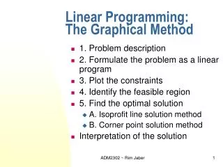
Graphical Solution of an LP Problem • Used to solve LP problems with two (and sometimes three) decision variables • Consists of two phases • Finding the values of the decision variables for which all the constraints are met (feasible region of the solution space) • Determining the optimal solution from all the points in the feasible region (from our knowledge of the nature of the optimal solution)
Finding the Feasible Region (2D) • Steps • Use the axis in a 2-dimensional graph to represent the values that the decision variables can take • For each constraint, replace the inequalities with equations and graph the resulting straight line on the 2-dimensional graph • For the inequality constraints, find the side (half-space) of the graph meeting the original conditions (evaluate whether the inequality is satisfied at the origin) • Find the intersection of all feasible regions defined by all the constraints. The resulting region is the (overall) feasible region.
Flair Furniture Company Data - Table 7.1 Available Hours This Week T Tables C Chairs Department • Carpentry • Painting • &Varnishing 4 2 3 1 240 100 Hours Required to Produce One Unit Mathematical formulation: Profit Amount $7 $5 Constraints: 4T + 3C 240 (Carpentry) 2T + 1C 100 (Paint & Varnishing) T ≥ 0 (1st nonnegative cons) C ≥ 0 (2nd nonnegative cons) Max. Objective, z: 7T + 5C
Flair Furniture Company Constraints The easiest way to solve a small LP problem, such as that of the Flair Furniture Company, is with the graphical solution approach. The graphical method works only when there are two decision variables, but it provides valuable insight into how larger problems are structured. When there are more than two variables, it is not possible to plot the solution on a two-dimensional graph; a more complex approach is needed. But the graphical method is invaluable in providing us with insights into how other approaches work.
Flair Furniture Company Constraints 120 100 80 60 40 20 0 Painting/Varnishing Number of Chairs Carpentry 20 40 60 80 100 2T + 1C ≤ 100 4T + 3C ≤ 240 Number of Tables
Flair Furniture Company Feasible Region 120 100 80 60 40 20 0 Painting/Varnishing Number of Chairs Carpentry Feasible Region 20 40 60 80 100 Number of Tables
Isoprofit Lines Steps 1. Graph all constraints and find the feasible region. 2. Select a specific profit (or cost) line and graph it to find the slope. 3. Move the objective function line in the direction of increasing profit (or decreasing cost) while maintaining the slope. The last point it touches in the feasible region is the optimal solution. 4. Find the values of the decision variables at this last point and compute the profit (or cost).
Flair Furniture Company Isoprofit Lines Isoprofit Line Solution Method • Start by letting profits equal some arbitrary but small dollar amount. • Choose a profit of, say, $210. - This is a profit level that can be obtained easily without violating either of the two constraints. • The objective function can be written as $210 = 7T + 5C.
Flair Furniture Company Isoprofit Lines Isoprofit Line Solution Method • The objective function is just the equation of a line called an isoprofit line. - It represents all combinations of (T, C) that would yield a total profit of $210. • To plot the profit line, proceed exactly as done to plot a constraint line: - First, let T = 0 and solve for the point at which the line crosses the C axis. - Then, let C = 0 and solve for T. • $210 = $7(0) + $5(C) • C = 42 chairs • Then, let C = 0 and solve for T. • $210 = $7(T) + $5(0) • T = 30 tables
Flair Furniture Company Isoprofit Lines Isoprofit Line Solution Method • Next connect these two points with a straight line. This profit line is illustrated in the next slide. • All points on the line represent feasible solutions that produce an approximate profit of $210 • Obviously, the isoprofit line for $210 does not produce the highest possible profit to the firm. • Try graphing more lines, each yielding a higher profit. • Another equation, $420 = $7T + $5C, is plotted in the same fashion as the lower line.
Flair Furniture Company Isoprofit Lines Isoprofit Line Solution Method • When T = 0, • $420 = $7(0) + 5(C) • C = 84 chairs • When C = 0, • $420 = $7(T) + 5(0) • T = 60 tables • This line is too high to be considered as it no longer touches the feasible region. • The highest possible isoprofit line is illustrated in the second following slide. It touches the tip of the feasible region at the corner point (T = 30, C = 40) and yields a profit of $410.
Flair Furniture Company Isoprofit Lines 120 100 80 60 40 20 0 Painting/Varnishing 7T + 5C = 210 Number of Chairs 7T + 5C = 420 Carpentry 20 40 60 80 100 Number of Tables
Flair Furniture Company Optimal Solution Isoprofit Lines 120 100 80 60 40 20 0 Painting/Varnishing Solution (T = 30, C = 40) Number of Chairs Carpentry 20 40 60 80 100 Number of Tables
Flair Furniture Company Corner Point Corner Point Solution Method • A second approach to solving LP problems • It involves looking at the profit at every corner point of the feasible region • The mathematical theory behind LP is that the optimal solution must lie at one of the corner points in the feasible region