Download
1 / 33
390 likes | 475 Views
Addressing Modes. Chapter 11 S. Dandamudi. Addressing modes Simple addressing modes Register addressing mode Immediate addressing mode Memory addressing modes 16-bit and 32-bit addressing Operand and address size override prefixes Direct addressing Indirect addressing Based addressing

E N D
Addressing Modes Chapter 11 S. Dandamudi
Addressing modes Simple addressing modes Register addressing mode Immediate addressing mode Memory addressing modes 16-bit and 32-bit addressing Operand and address size override prefixes Direct addressing Indirect addressing Based addressing Indexed addressing Based-indexed addressing Examples Sorting (insertion sort) Binary search Arrays One-dimensional arrays Multidimensional arrays Examples Sum of 1-d array Sum of a column in a 2-d array Recursion Examples Outline S. Dandamudi
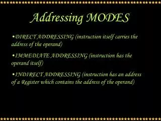
Addressing Modes • Addressing mode refers to the specification of the location of data required by an operation • Pentium supports three fundamental addressing modes: • Register mode • Immediate mode • Memory mode • Specification of operands located in memory can be done in a variety of ways • Mainly to support high-level language constructs and data structures S. Dandamudi
Pentium Addressing Modes (32-bit Addresses) S. Dandamudi
Memory Addressing Modes (16-bit Addresses) S. Dandamudi
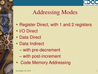
Simple Addressing Modes • Register addressing mode • Operands are located in registers • It is the most efficient addressing mode • Immediate addressing mode • Operand is stored as part of the instruction • This mode is used mostly for constants • It imposes several restrictions • Efficient as the data comes with the instructions • Instructions are generally prefetched • Both addressing modes are discussed before • See Chapter 9 S. Dandamudi
Memory Addressing Modes • Pentium offers several addressing modes to access operands located in memory • Primary reason: To efficiently support high-level language constructs and data structures • Available addressing modes depend on the address size used • 16-bit modes (shown before) • same as those supported by 8086 • 32-bit modes (shown before) • supported by Pentium • more flexible set S. Dandamudi
32-Bit Addressing Modes • These addressing modes use 32-bit registers Segment + Base + (Index * Scale) + displacement CS EAX EAX 1 no displacement SS EBX EBX 2 8-bit displacement DS ECX ECX 4 32-bit displacement ES EDX EDX 8 FS ESI ESI GS EDI EDI EBP EBP ESP S. Dandamudi
Differences between 16- and 32-bit Modes 16-bit addressing 32-bit addressing Base register BX, BP EAX, EBX, ECX, EDX, ESI, EDI, EBP, ESP Index register SI, DI EAX, EBX, ECX, EDX, ESI, EDI, EBP Scale factor None 1, 2, 4, 8 Displacement 0, 8, 16 bits 0, 8, 32 bits S. Dandamudi
16-bit or 32-bit Addressing Mode? • How does the processor know? • Uses the D bit in the CS segment descriptor D = 0 • default size of operands and addresses is 16 bits D = 1 • default size of operands and addresses is 32 bits • We can override these defaults • Pentium provides two size override prefixes 66H operand size override prefix 67H address size override prefix • Using these prefixes, we can mix 16- and 32-bit data and addresses S. Dandamudi
Examples: Override Prefixes • Our default mode is 16-bit data and addresses Example 1: Data size override mov AX,123 ==> B8 007B mov EAX,123 ==> 66 | B8 0000007B Example 2: Address size override mov AX,[EBX*ESI+2] ==> 67 | 8B0473 Example 3: Address and data size override mov EAX,[EBX*ESI+2] ==> 66 | 67 | 8B0473 S. Dandamudi
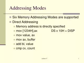
Memory Addressing Modes • Direct addressing mode • Offset is specified as part of the instruction • Assembler replaces variable names by their offset values • Useful to access only simple variables Example total_marks = assign_marks + test_marks + exam_marks translated into mov EAX,assign_marks add EAX,test_marks add EAX,exam_marks mov total_marks,EAX S. Dandamudi
Memory Addressing Modes (cont’d) • Register indirect addressing mode • Effective address is placed in a general-purpose register • In 16-bit segments • only BX, SI, and DI are allowed to hold an effective address add AX,[BX] is valid add AX,[CX] is NOT allowed • In 32-bit segments • any of the eight 32-bit registers can hold an effective address add AX,[ECX] is valid S. Dandamudi
Memory Addressing Modes (cont’d) • Default Segments • 16-bit addresses • BX, SI, DI : data segment • BP, SP : stack segment • 32-bit addresses • EAX, EBX, ECX, EDX, ESI, EDI: data segment • EBP, ESP: stack segment • Possible to override these defaults • Pentium provides segment override prefixes S. Dandamudi
Based Addressing • Effective address is computed as base + signed displacement • Displacement: • 16-bit addresses: 8- or 16-bit number • 32-bit addresses: 8- or 32-bit number • Useful to access fields of a structure or record • Base register points to the base address of the structure • Displacement relative offset within the structure • Useful to access arrays whose element size is not 2, 4, or 8 bytes • Displacement points to the beginning of the array • Base register relative offset of an element within the array S. Dandamudi
Based Addressing (cont’d) S. Dandamudi
Indexed Addressing • Effective address is computed as (index * scale factor) + signed displacement • 16-bit addresses: • displacement: 8- or 16-bit number • scale factor: none (i.e., 1) • 32-bit addresses: • displacement: 8- or 32-bit number • scale factor: 2, 4, or 8 • Useful to access elements of an array (particularly if the element size is 2, 4, or 8 bytes) • Displacement points to the beginning of the array • Index register selects an element of the array (array index) • Scaling factor size of the array element S. Dandamudi
Indexed Addressing (cont’d) Examples add AX,[DI+20] • We have seen similar usage to access parameters off the stack (in Chapter 10) add AX,marks_table[ESI*4] • Assembler replaces marks_table by a constant (i.e., supplies the displacement) • Each element of marks_table takes 4 bytes (the scale factor value) • ESI needs to hold the element subscript value add AX,table1[SI] • SI needs to hold the element offset in bytes • When we use the scale factor we avoid such byte counting S. Dandamudi
Based-Indexed Addressing Based-indexed addressing with no scale factor • Effective address is computed as base + index + signed displacement • Useful in accessing two-dimensional arrays • Displacement points to the beginning of the array • Base and index registers point to a row and an element within that row • Useful in accessing arrays of records • Displacement represents the offset of a field in a record • Base and index registers hold a pointer to the base of the array and the offset of an element relative to the base of the array S. Dandamudi
Based-Indexed Addressing (cont’d) • Useful in accessing arrays passed on to a procedure • Base register points to the beginning of the array • Index register represents the offset of an element relative to the base of the array Example Assuming BX points to table1 mov AX,[BX+SI] cmp AX,[BX+SI+2] compares two successive elements of table1 S. Dandamudi
Based-Indexed Addressing (cont’d) Based-indexed addressing with scale factor • Effective address is computed as base + (index * scale factor) + signed displacement • Useful in accessing two-dimensional arrays when the element size is 2, 4, or 8 bytes • Displacement ==> points to the beginning of the array • Base register ==> holds offset to a row (relative to start of array) • Index register ==> selects an element of the row • Scaling factor ==> size of the array element S. Dandamudi
Illustrative Examples • Insertion sort • ins_sort.asm • Sorts an integer array using insertion sort algorithm • Inserts a new number into the sorted array in its right place • Binary search • bin_srch.asm • Uses binary search to locate a data item in a sorted array • Efficient search algorithm S. Dandamudi
Arrays One-Dimensional Arrays • Array declaration in HLL (such as C) int test_marks[10]; specifies a lot of information about the array: • Name of the array (test_marks) • Number of elements (10) • Element size (2 bytes) • Interpretation of each element (int i.e., signed integer) • Index range (0 to 9 in C) • You get very little help in assembly language! S. Dandamudi
Arrays (cont’d) • In assembly language, declaration such as test_marks DW 10 DUP (?) only assigns name and allocates storage space. • You, as the assembly language programmer, have to “properly” access the array elements by taking element size and the range of subscripts. • Accessing an array element requires its displacement or offset relative to the start of the array in bytes S. Dandamudi
To compute displacement, we need to know how the array is laid out Simple for 1-D arrays Assuming C style subscripts displacement = subscript * element size in bytes If the element size is 2, 4, or 8 bytes a scale factor can be used to avoid counting displacement in bytes Arrays (cont’d) S. Dandamudi
Multidimensional Arrays • We focus on two-dimensional arrays • Our discussion can be generalized to higher dimensions • A 53 array can be declared in C as int class_marks[5][3]; • Two dimensional arrays can be stored in one of two ways: • Row-major order • Array is stored row by row • Most HLL including C and Pascal use this method • Column-major order • Array is stored column by column • FORTRAN uses this method S. Dandamudi
Multidimensional Arrays (cont’d) S. Dandamudi
Multidimensional Arrays (cont’d) • Why do we need to know the underlying storage representation? • In a HLL, we really don’t need to know • In assembly language, we need this information as we have to calculate displacement of element to be accessed • In assembly language, class_marks DW 5*3 DUP (?) allocates 30 bytes of storage • There is no support for using row and column subscripts • Need to translate these subscripts into a displacement value S. Dandamudi
Multidimensional Arrays (cont’d) • Assuming C language subscript convention, we can express displacement of an element in a 2-D array at row i and column j as displacement = (i * COLUMNS + j) * ELEMENT_SIZE where COLUMNS = number of columns in the array ELEMENT_SIZE = element size in bytes Example: Displacement of class_marks[3,1] element is (3*3 + 1) * 2 = 20 S. Dandamudi
Examples of Arrays Example 1 • One-dimensional array • Computes array sum (each element is 4 bytes long e.g., long integers) • Uses scale factor 4 to access elements of the array by using a 32-bit addressing mode (uses ESI rather than SI) • Also illustrates the use of predefined location counter $ Example 2 • Two-dimensional array • Finds sum of a column • Uses “based-indexed addressing with scale factor” to access elements of a column S. Dandamudi
Recursion • A recursive procedure calls itself • Directly, or • Indirectly • Some applications can be naturally expressed using recursion factorial(0) = 1 factorial (n) = n * factorial(n-1) for n > 0 • From implementation viewpoint • Very similar to any other procedure call • Activation records are stored on the stack S. Dandamudi
Recursion (cont’d) S. Dandamudi
Recursion (cont’d) • Example 1 • Factorial • Discussed before • Example 2 • Quicksort (on an N-element array) • Basic algorithm • Selects a partition element x • Assume that the final position of x is array[i] • Moves elements less than x into array[0]…array[i-1] • Moves elements greater than x into array[i+1]…array[N-1] • Applies quicksort recursively to sort these two subarrays Last slide S. Dandamudi