Download

1 / 31
320 likes | 463 Views
In-silico Implementation of Bacterial Chemotaxis. Lin Wang Advisor: Sima Setayeshgar. Chemotaxis in E. coli. Dimensions: Body size: 1 μ m in length 0.4 μ m in radius Flagellum: 10 μ m long. From Berg Lab. From R. M. Berry, Encyclopedia of Life Sciences.

E N D
In-silico Implementation of Bacterial Chemotaxis Lin Wang Advisor: Sima Setayeshgar
Chemotaxis in E. coli Dimensions: Body size: 1 μm in length 0.4 μm in radius Flagellum: 10 μm long From Berg Lab From R. M. Berry, Encyclopedia of Life Sciences Physical constants: Cell speed: 20-30 μm/sec Mean run time: 1 sec Mean tumble time: 0.1 sec
From Single Cells to Populations … Chemotactic response of individual cells forms the basis of macroscopic pattern formation in populations of bacteria: Colonies Biofilms Pattern formation in E. coli: From H.C. Berg and E. O. Budrene, Nature (1995) Agrobacterium biofilm: From Fuqua Lab
Motivation • Chemotaxis as a well-characterized “model” signaling network, amenable to quantitative analysis and extension to other signaling networks from the standpoint of general information-processing concepts, such as signal to noise, adaptation and memory • Chemotaxis as an important biophysical mechanism, for example underlying initial stages of biofilm formation
Modeling Chemotaxis in E.coli Stimulus Signal Transduction Pathway [CheY-P] Motor Response Flagellar Response Motion
Outline • Chemotaxis signal transduction network in E. coli • Stochastic implementation of reaction network using Stochsim • Flagellar and motor response • Preliminary numerical results
Ligand Binding E: receptor complex a: ligand (eg., aspartate) Rapid equilibrium: Rates1: E: KD = 1.71x10⁻⁶ M-1 E*: KD = 12x10-6 M-1 [1] Morton-Firth et al., J. Mol. Biol.(1999)
Receptor Activation En: methylated receptor complex; activation probability, P1(n) Ena: ligand-bound receptor complex; activation probability, P2(n) En*: active form of En En*a: active form of Ena Table 1: Activation Probabilities
Methylation (1) (2) R: CheR En(a): En, Ena En(*)(a): En, En*,Ena, En*a Rate constants: k1f = 5x10⁶ M-1sec-1 k1r = 1 sec-1 k2f = 0.819 sec-1
Demethylation (1) (2) Bp: CheB-P En*(a): En*, En*a Rate constants: k1f = 1x10⁶ M-1sec-1 k1r = 1.25 sec-1 k2f = 0.15484 sec-1
Autophosphorylation E*: En*, En*a Rate constant: kf = 15.5 sec-1
CheY Reactions Y: CheY Yp: CheY-P Rate constants: k1f = 1.24x10⁻³ sec-1 k1r = 4.5x10⁻² sec-1 k2f = 14.15 sec-1
CheY Phosphotransfer Rate constants: k1f = 5x10⁶ M-1sec-1 k2f = 20 sec-1 k2r = 5x10⁶ M-1sec-1 k3f = 7.5 sec-1 k3r = 5x10⁶ M-1sec-1
CheB Reactions B: CheB Bp: CheB-P Rate constant: kf = 0.35 sec-1
CheB Phosphotransfer Rate constants: k1f = 5x10⁶ M-1sec-1 k2f = 16 sec-1 k2r = 5x10⁶ M-1sec-1 k3f = 16 sec-1 k3r = 5x10⁶ M-1sec-1
Simulating Reactions Stochastic2:Reaction has probability P of occurring a) Generate x, a uniform random number in [0, 1]. b) x <= P, reaction happens. c) x > P, reaction does not happen. How to generate P from reaction rates? [2] Morton-Firth et al., J. Mol. Biol. (1998) Two methods: Deterministic: ODE description, using rate constants,
Stochsim Package Stochsim package is a general platform for simulating reactions using a stochastic method.
Pseudo-molecule Pseudo-molecules are used to simulate unimolecular reaction. Number of pseudomolecule in simulating system: k1max: fastest unimolecular reaction rate k2max: fastest bimolecular reaction rate
From Rate Constant to Probability • Unimolecular reaction • Bimolecular reaction • n: number of molecules from reaction system • n0: number of pseudomolecules • NA: Avogadro constant
Simulation Parameters Reaction Volume: 1.41 x 10⁻¹⁵ liter Rate constants given above. Table 2: Initial Numbers of Molecules
Output of Signal Transduction Network Fig 1. Number of CheY-P molecules as a function of time, the trace is smoothed by an averaging window of 0.3 sec. The motor switches state whenever threshold (red line) is crossed. It’s assumed that there is only 1 motor/cell.
Flagellar Response • Flagellar state directly reflects motor state, except that 20% of the motor changing from CCW to CW is dropped3. • Assume there is only 1 flagellum/cell. [3] Alon et al., The EMBO Journal (1998)
Motion • Motion of the cell is determined by the state of flagellum. CCW run CW tumble
t t+Δt α Run and Tumble Process • Run4 • Tumble5 v = 20 μm/s Dr = 0.06205 s-1 γ = 4 μ = -4.6 β = 18.32 [4] Zou et al., Biophys. J. (2003) [5] Berg and Brown, Nature (1972)
Some Simulation Results • Distribution of run and tumble intervals. • Diffusion of a population of cells in an unbounded region in the absence of stimulus. • Diffusion of a population of cells in a bounded region (z>0), with and without stimulus.
Motor CW and CCW Intervals Fig 2. Fraction of motor CW/CCW intervals of wild-type cell in an environment without ligand. Left: Experiment (Korobkova et al., Nature 2004); Right: Simulation
Diffusion in Unbounded Region: No Stimulus Fig 3. Mean-squared distance from initial position as a function of time (averaged over 540 cells). Diffusion constant is found to be 4.4 * 10-4 mm2/s, consistent with experimental results6. [6] Paul Lewus et al., BioTech. and BioEng. (2001)
Diffusion in Bounded Region (z>0) Fig 4. Number of cells (out of a total of 540) above z=1.2 mm as a function of time. Red: constant linear gradient of aspartate 10-8 zM/μM; Blue: no aspartate.
Future Directions Realistic description of chemotaxis in E. coli to explore: • Optimal biochemical signal processing (role of “adaptive” network adaptation time) • Role of chemotaxis in initial stages of biofilm formation