Download

1 / 64
640 likes | 713 Views
3. National Income: Where it Comes From and Where it Goes. The production function. denoted Y = F ( K , L ) shows how much output ( Y ) the economy can produce from Factor of Production: K units of capital and L units of labor reflects the economy’s level of technology

E N D
3 National Income:Where it Comes From and Where it Goes
The production function • denoted Y = F(K,L) • shows how much output (Y) the economy can produce from • Factor of Production:Kunits of capital and Lunits of labor • reflects the economy’s level of technology • exhibits constant returns to scale CHAPTER 3 National Income
Returns to scale: A review Initially Y1= F(K1,L1 ) Scale all inputs by the same factor z: K2 = zK1 and L2 = zL1 (e.g., if z = 1.25, then all inputs are increased by 25%) What happens to output, Y2 = F (K2,L2)? • If constant returns to scale, Y2 = zY1 • If increasing returns to scale, Y2 > zY1 • If decreasing returns to scale, Y2 < zY1 CHAPTER 3 National Income
Example 1 constant returns to scale for any z > 0 CHAPTER 3 National Income
Example 2 decreasing returns to scale for any z > 1 CHAPTER 3 National Income
Example 3 increasing returns to scale for any z > 1 CHAPTER 3 National Income
Now you try… • Determine whether constant, decreasing, or increasing returns to scale for each of these production functions: (a) (b) CHAPTER 3 National Income
Answer to part (a) constant returns to scale for any z > 0 CHAPTER 3 National Income
Answer to part (b) constant returns to scale for any z > 0 CHAPTER 3 National Income
The distribution of national income • determined by factor prices, the prices per unit that firms pay for the factors of production • wage = price of L • rental rate = price of K CHAPTER 3 National Income
Notation W = nominal wage R = nominal rental rate P = price of output W/P = real wage (measured in units of output) R/P = real rental rate CHAPTER 3 National Income
How factor prices are determined • Supply of each factor is fixed. • Assume markets are competitive: each firm takes W, R, and P as given. • Basic idea:A firm hires each unit of labor if the cost does not exceed the benefit. • cost = real wage • benefit = marginal product of labor CHAPTER 3 National Income
Marginal product of labor (MPL) • definition:The extra output the firm can produce using an additional unit of labor (holding other inputs fixed): MPL = F(K,L+1) – F(K,L)=W/P Since we assume the production function exhibits Constant return to scale, we can assume it as CHAPTER 3 National Income
MPL 1 As more labor is added, MPL MPL 1 Slope of the production function equals MPL 1 MPL and the production function Y output MPL L labor CHAPTER 3 National Income
Diminishing marginal returns • As a factor input is increased, its marginal product falls (other things equal). • Intuition:Suppose L while holding K fixed fewer machines per worker lower worker productivity CHAPTER 3 National Income
Check your understanding: • Which of these production functions have diminishing marginal returns to labor? CHAPTER 3 National Income
Units of output Real wage MPL, Labor demand Units of labor, L Quantity of labor demanded MPL and the demand for labor Each firm hires labor up to the point where MPL = W/P. CHAPTER 3 National Income
Labor supply Units of output equilibrium real wage MPL, Labor demand Units of labor, L The equilibrium real wage The real wage adjusts to equate labor demand with supply. CHAPTER 3 National Income
Determining the rental rate We have just seen that MPL= W/P. The same logic shows that MPK= R/P: • diminishing returns to capital: MPK as K • The MPKcurve is the firm’s demand curve for renting capital. • Firms maximize profits by choosing Ksuch that MPK = R/P. CHAPTER 3 National Income
Units of output Supply of capital equilibrium R/P MPK, demand for capital Units of capital, K The equilibrium real rental rate The real rental rate adjusts to equate demand for capital with supply. CHAPTER 3 National Income
The Neoclassical Theory of Distribution • states that each factor input is paid its marginal product • is accepted by most economists CHAPTER 3 National Income
nationalincome capitalincome laborincome How income is distributed: total labor income = total capital income = If production function has constant returns to scale, then CHAPTER 3 National Income
The ratio of labor income to total income in the U.S. Labor’s share of total income Labor’s share of income is approximately constant over time.(Hence, capital’s share is, too.) CHAPTER 3 National Income
The Cobb-Douglas Production Function • The Cobb-Douglas production function has constant factor shares: = capital’s share of total income: capital income = MPK x K = Y labor income = MPL x L = (1 – )Y • The Cobb-Douglas production function is: where A represents the level of technology. CHAPTER 3 National Income
The Cobb-Douglas Production Function • Each factor’s marginal product is proportional to its average product: CHAPTER 3 National Income
Demand for goods & services Components of aggregate demand: C = consumer demand for g & s I = demand for investment goods G = government demand for g & s (closed economy: no NX ) CHAPTER 3 National Income
Consumption, C • def: Disposable income is total income minus total taxes: Y – T. • Consumption function: C = C(Y – T) Shows that (Y – T) C • def: Marginal propensity to consume (MPC)is the increase in C caused by a one-unit increase in disposable income. CHAPTER 3 National Income
C C(Y –T ) The slope of the consumption function is the MPC. MPC 1 Y – T The consumption function CHAPTER 3 National Income
Investment, I • The investment function is I= I(r), where r denotes the real interest rate,the nominal interest rate corrected for inflation. • The real interest rate is • the cost of borrowing • the opportunity cost of using one’s own funds to finance investment spending. So, r I CHAPTER 3 National Income
r Spending on investment goods depends negatively on the real interest rate. I(r) I The investment function CHAPTER 3 National Income
Government spending, G • G = govt spending on goods and services. • G excludes transfer payments (e.g., social security benefits, unemployment insurance benefits). • Assume government spending and total taxes are exogenous: CHAPTER 3 National Income
The market for goods & services • Aggregate demand: • Aggregate supply: • Equilibrium: • The real interest rate adjusts to equate demand with supply. CHAPTER 3 National Income
The loanable funds market • A simple supply-demand model of the financial system. • One asset: “loanable funds” • demand for funds: investment • supply of funds: saving • “price” of funds: real interest rate CHAPTER 3 National Income
r I(r) I Loanable funds demand curve The investment curve is also the demand curve for loanable funds. CHAPTER 3 National Income
Supply of funds: Saving • The supply of loanable funds comes from saving: • Households use their saving to make bank deposits, purchase bonds and other assets. These funds become available to firms to borrow to finance investment spending. • The government may also contribute to saving if it does not spend all the tax revenue it receives. CHAPTER 3 National Income
Types of saving private saving = (Y – T) – C public saving = T – G national saving, S = private saving + public saving = (Y –T ) – C + T – G = Y – C – G CHAPTER 3 National Income
digression: Budget surpluses and deficits • If T > G, budget surplus = (T – G) = public saving. • If T < G, budget deficit = (G – T)and public saving is negative. • If T = G, “balanced budget,” public saving = 0. • The U.S. government finances its deficit by issuing Treasury bonds – i.e., borrowing. CHAPTER 3 National Income
U.S. Federal Government Surplus/Deficit, 1940-2004 CHAPTER 3 National Income
U.S. Federal Government Debt, 1940-2004 Fact: In the early 1990s, about 18 cents of every tax dollar went to pay interest on the debt. (Today it’s about 9 cents.) CHAPTER 3 National Income
四、當前經濟面臨的挑戰 5.財政收支惡化,債台高築(1)1991年度至1999年度間,中央政府債務餘額由2169億元增至1兆2149億元, 平均債務餘額年增1248億元。(2)2000年度因凍省納編原省府債務8139億元,致中央政府債務餘額激增至2兆 3575億元。(3)依據政府編列2004年度中央政府總預算案,截至2004年度止中央政府債務餘 額將達3兆4290億元,較2000年度擴增1兆715億元,四年來平均每年增加2678億 元,為前8年之2.2倍。。 億元 年度 CHAPTER 3 National Income 29
中國時報 2007.10.01近10年 每人增加11萬負債本報訊 選舉烽火連年燒遍全台,面對明年將改朝換代的超級選舉,朝野政黨殺紅了眼,為搶選票,無所不用其極,由陳水扁總統以降,左手加碼提高各項福利津貼,右手釋放減稅利多。國家財政大失血,近十年來債台高築,平均每人增加負債十一萬元,民調更顯示已有五三%的民眾擔心財政破產。 稅收雖超徵 債務卻有增無減 過去十年,台灣政局以前所未見的速度重組更迭,債務也如滾雪球般越滾越大。據財政部統計,中央政府累計的未償債務總額由八七年的一.三七兆,至今年八月初已快速攀升到三.八七兆的新高;如加上地方政府債務餘額,就達四兆四七七四億元。中央政府債務未償餘額佔GNP比例,由一三.八五%銳增到三一.○四%,暴增逾一倍。即使這兩年政府稅收都有超徵,債務卻有增無減,引來國際信評機構頻頻示警。 如果不計地方政府六千多億元的負債,單中央政府債務,每個人平均為政府背負的負債金額,七十六年時只有四千多元,八十年破萬到一萬二千多元,八十六年接近六萬元,接著十年就「勢如破竹」,一路提高到現在的近十七萬元。而此債務增加的速度,正與台灣政局進入政黨競爭白熱化、政客爭相「搞肉桶」完全契合。 前財政部次長、中信證董事長陳沖直言,各級政府債務飛快成長的趨勢「蠻可怕的」,趨勢背後領導人透露的心態更讓國家置於險地,「政府若對債務增加的速度缺乏警覺,以為還可以大肆揮霍浪費的話,這種心態不改就很危險」。 與民國八十九年底,約二兆七千餘億元的水位相比,台灣政府債務大幅增加一兆七千餘億元。國內財政日益惡化,政大財研所教授曾巨威直言,問題出在「國家財政收入與支出面都出了狀況」。 鈔票換選票 大慷國庫之慨 以收入面而言,曾巨威指出,在政治選舉效應下,政治人物慷國庫之慨,開出逾千億的減稅支票,但近半世紀以來,立院僅在去年通過「最低稅負制」,為國庫每年增加約一六○億的微薄稅收;再論支出面,隨社會結構轉型,社福支出倍數成長,加上政府花錢無效率,如蚊子館、蚊子機場等到處林立,在在都讓國家財政雪上加霜。 伴隨民主化近程開展,國內幾乎年年有選舉,
國家資產遭受偷竊浪費項目與因而損失或耗費的金額(中國時報台灣希望專題系列之四─被偷竊的國家/工商時報 2007.10.02) • 核四貿然停建損失估計2393億至4000億元 • 實施油電價補貼損失1630億元 • 公營行庫轉銷呆帳與對問題企業紓困耗費8000億元 • 調降金融業營業稅支援金融機構打消呆帳耗費2200億元 • 為經營不良及問題金融機構善後組建金融重建基金耗費4000億元 • 機場興建與整修動用415億元(二十五縣市建設了十八座機場,創下全球機場密度最高的笑話) • 機場營運虧損106億元 • 四十餘年來利用租稅優惠獎勵特定企業耗費一兆元左右 • 監理不善給予上市櫃公司掏空機會不法所得高達947億元等 • 蚊子館到處林立
中國時報 2007.10.01政客樂此不疲「蚊子館」蓋不完本報訊 選舉機場、蚊子館,這個故事還未結束,而且仍在繼續發生中。因年年有選舉,大大小小的「蚊子館」不停地產生,政客樂此不疲。 去年十月間,趕著在年底北高市長選舉前,經濟部及經建會緊急通過「高雄世界貿易中心暨國際會議中心」可行性評估,及「高雄軟體科技園區加速發展計畫」兩項大計畫,前者要花政府三十億元,後者則使政府短少租金八千萬元。 目前國內已有世貿展覽館及正在興建的南港展覽館,而外貿協會董事長許志仁一直爭取在桃園新設國際級五千個攤位以上的大型展覽館,但究竟國內有無如此大的展覽需求,經濟部及行政院內部多有討論,並無定案。但突然間,卻冒出了「高雄世界貿易中心暨國際會議中心」,落腳在高雄。 面對媒體追問,國貿局執行秘書鍾興國表示,這個案子由民間開發不具可行性,整體財務計畫淨現值均為負數,且投資報酬率在一.五%以下,只能由政府興建,他也坦承,高雄市世貿中心及會議中心「剛開始可能會成為蚊子館,」他接著又補充說,但政府會找有能力的廠商舉辦大型展覽,並提供多功能用途,增加使用效益,例如結合演唱會、表演等,以保持彈性。鍾國興指出,到民國一一一年,使用率就會達四○%。 一項投資三十億元,十多年後使用率才會到達四○%,擺明就是「蚊子館」,但經濟部得做,經建會得快速通過,文官都清楚,也很無奈,一切都是為選舉。 今年,政府撒紅包的情況更嚴重。行政院在九月初一口氣通過,在民國一百年前,投入三○二億元,要在中南部興建歌劇院、文化中心等設施,包括:台中大都會歌劇院、國家數位圖書館、台灣工藝文化園區、故宮南院分院、台灣歷史博物館、衛武營藝術文化中心、高雄流行音樂中心、以及中部及南部表演藝術發展計畫。 政府美其名是要將文化建設向中南部延伸,甚至延伸至離島、東部等地設美術館及文化創意園區。在這些大型文化建設中,最大的一項是高雄的衛武營藝術文化中心,高達八十三億元,預估一○一年可以完成。 《阿房宮賦》結語說:「秦人不暇自哀,而後人哀之;後人哀之而不鑑之,亦使後人復哀後人也。」大概,就是這麼一回事吧!
選舉機場養蚊子 世界奇觀本報訊 台灣是選舉國家,為了選舉,造就了許多為選票而出生的「選舉機場」。廿五縣市有十八座機場,密度世界第一。屏東縣境內,相距數十公里,就有兩座機場,最是受關愛。 交通決策官員不諱言說,「很多機場的核定,都是在選舉前,機場營運也是配合選舉。」例如,屏東機場正是在九一年立委選舉前一年底核定,花了十五億元蓋航站;而花了五億元整建的恆春機場與花蓮機場新航站、台中清泉崗機場,則都趕在九三年總統選舉前營運;真是趕得早不如趕得巧。 政院壓著同意 經建會難擋 「這兩個機場,當時的經建會都擋了許久,因為高鐵一通車,屏東機場完全沒有機會,而恆春機場則有落山風,且航道在核三廠上方,這些當時都有紀錄。」這位官員透露,「後來都是被行政院壓著同意。」 也因為政治掛帥、專業殿後、審查機制淪喪,類似的因選票而產生的「養蚊子」機場不斷增加。根據統計,清泉崗機場的使用率還有四成六,說起來並非殿後,花蓮機場更只有十九%;最誇張者當屬恆春機場五%,屏東機場也不過七%。而今年高鐵通車,預估西部走廊航空運量將減少一半,西部機場使用率將呈溜滑梯直線下降。
中國時報 2007.10.01政商一家親 藍綠均須檢驗本報訊 在前有泰公、後有小馬下,政商一家親,呆帳大戶不愁。十年來的紓困政策,就讓泛公股行庫吞下近四千億元的呆帳,平均台灣每人被迫要幫逾一千四百名呆帳大戶還債一萬五千元。如果再加上另外轉銷的四千億元呆帳,咱們為「帳多不愁」的借款人,還得可多的呢! CHAPTER 3 National Income
中國時報 2007.10.01舉債近五百億 苦撐低廉水價本報訊 在政府「德政」下,台灣一噸自來水比一瓶礦泉水便宜!但,這卻是犧牲應有的盈餘、靠舉債近五百億元撐出的「德政」。 為提高供水普及率,自來水公司每年均需投入鉅資辦理各項自來水工程建設,由於水價長期接近成本,致無法累積自有資金投資建設,致水公司長年以舉債度日,至九十五年底借款餘額為四七四.七一億元。 台灣的水,有多便宜?經建會主委何美玥曾形容,一般家庭中的浴缸裝滿水是○.二三公噸,裝滿四個缸是一公噸,才賣一○.七元。「這比超商賣一瓶礦泉水都不如。」國內水價長期偏低,台灣省平均一噸為一○.七元,台北市更便宜,一噸只有七元,國營會官員表示,因水價長年未調,成本早就超過售價。 CHAPTER 3 National Income
中國時報 2007.10.01政府倒貼油價 形同劫貧濟富本報訊 什麼是用油補貼?中油董事長潘文炎說,「用油少的補貼用油多的,不開車的補貼開車的,貧者補貼富者,虧損由全民埋單。」它是標準的劫貧濟富。 九三年中油賺了一六○億元,九四年稅前盈餘滑落至八十三億元,而去年更大虧一八八億元。經濟部官員解釋,去年謝長廷擔任行政院長時強勢介入油價,因而造成中油大虧一八八億元,但之前,政府也是刻意壓低油價,「只是介入方式不像謝長廷那麼大張旗鼓。」 潘文炎直言,中油資本額不過一三○一億元,若取消浮動油價制,硬要中油苦撐,中油一年就得虧六百億元,「不到三年,中油就倒店!」 CHAPTER 3 National Income
中國時報 2007.10.01核四輕率停建 四千億瞬間蒸發本報訊 那天,陳總統與當時國民黨主席連戰會面後,當時的行政院長張俊雄就宣布核四停建。外界說,這是打了連戰一巴掌,錯了!這巴掌,是打在全民臉上,這一掌,價值連城;造成的損失,至少二三九三億元,多則可能高達四千億元,也就是說,全台每戶家庭因這項錯誤決策,被政府A走了至少三萬元。 政黨輪替、民進黨上台後,祭出「神主牌」,以四個月簡單的幕僚作業、草率評估後,宣布停建核四。 但台灣真的能承受停建核四,其他核電廠提早除役的衝擊嗎?答案是否定的。停建核四政策宣布一一○天後,執政者還是得向現實環境低頭,重建核四。只是短短百餘天的政策轉向,已讓國庫嚴重失血。 CHAPTER 3 National Income
10年來 稅都白繳了中國時報 2007.10.01 去年台灣的個人綜合所得稅收三三四三億元,八十六年是二○六二億元,十年平均值二四九八億元;因此,如果這一切未發生,你可以七年多不繳稅! 至於每年預算在五千到八千億元之譜的公共建設投資,更是一個隱形、難以估算的黑洞。各地林立的「選舉機場」、蚊子館、三步一漁港的離島建設、過度華麗的法院與政府機關…,都說明了有多少資源被浪費、被虛擲;而上至部會政務官、立委,下至鄉鎮地方首長及公務員,牽扯的貪瀆司法案件之多,更讓人難以想像國庫被偷竊的金額,更甭談計算了。 民進黨執政前曾批評國民黨,每年至少A走公共建設一成以上的經費,算算是七百億元左右;民進黨執政七年了,貪瀆案與浪費程度,就算未「青出於藍」,但至少是「前後輝映,不遑多讓」。這筆錢,也是五千到七千億元以上。 CHAPTER 3 National Income