CDMA NETWORK PLAN AND OPTIMIZE

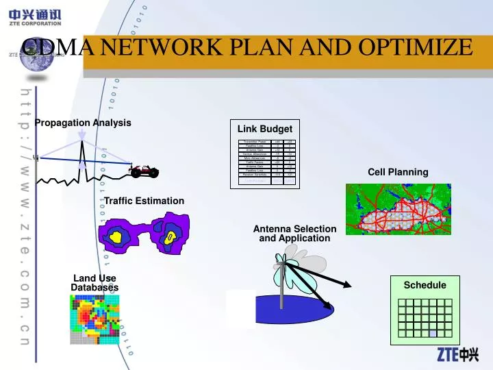
1. Propagation Analysis Link Budget Transmitter Power +44 +22 Feedline Loss -3 0 Antenna Gain +12 0 Various Allowances -15 -14 More Allowances -8 -8 Traffic Factors +20 0 Antenna Gain 0 +12 Cell Planning Feedline Loss 0 -3 Receiver Sensitivity -116 -121 Link Budget 135.4 140.2 Traffic Estimation Antenna Selection and Application Land Use Databases Schedule CDMA NETWORK PLAN AND OPTIMIZE

2. CDMA NETWORK PLAN AND OPTIMIZE • RF Propagation • underlying mechanisms • modeling and prediction • Antenna Principles and Applications • basic physics and operation • application issues • commercial products • Traffic Engineering • dimensioning • backhaul and NETWORKworking considerations • Technology-Specific Subjects • Application principles, rules, limits, guidelines • Hardware Architecture and Capabilities

3. -40 -50 -60 -70 RSSI, dBm -80 -90 -100 , dB -110 4 8 12 16 20 24 28 32 0 Distance from Cell Site, km measured signal Okumura-Hata model CDMA NETWORK PLAN AND OPTIMIZE

4. CDMA NETWORK PLAN AND OPTIMIZE • Section A: Propagation Basics • Radio Links: Types, key elements, configurations • Frequency and Wavelength; the RF spectrum • Section B: Overview of Propagation Mechanisms • Free-Space, Reflection/Cancellation, Knife-Edge Diffraction • Additional modes and real-life complications, multipath • Techniques for combating multipath fading • Section C: Propagation Models • Okumura-Hata, COST-231, Walfisch Ikegami • Confidence factors and statistical distribution • Link Budgets • Section D: Overview of Measurement Tools & Methods • Section E: Overview of Propagation Prediction Tools

5. CDMA NETWORK PLAN AND OPTIMIZE Section A Objectives • Recognize the basic principles of RF propagation • Identify key elements in radio links • Recognize the possible configurations for radio links • Understand the role of frequency in propagation • Remember the wavelength of the signals of your own communications system • Mathematic tools • Total considerations

6. Antenna 1 Antenna 2 ElectromagNETWORKic Fields Transmission Line Transmission Line Trans- mitter Receiver Information Information current Propagation current Propagation: Basic Elements of a Radio Link • Propagation is the science of how radio signals travel (propagate from one transmitting antenna to another receiving antenna • Propagation is an unavoidable part of every radio link • To successfully design just one radio link, or a whole wireless system, one must understand how propagation occurs • basic mechanics of the propagation process • appropriate models/techniques for propagation prediction • characteristics of the other components of the overall radio link

7. power output • modulation type • spectral density • coding, if any Transmitter Trans. Line • line loss • gain, bandwidth • beamwidth • polarization Antenna • path loss • gain, bandwidth • beamwidth • polarization Antenna Trans. Line • line loss • sensitivity • selectivity • spreading gain • coding gain • dynamic range Receiver Elements and Parameters of a Radio Link • Transmitter • Generates RF energy on a desired frequency • Modulates the RF energy to convey information • Antennas • Convert RF energy into electromagnetic fields, vice versa • Focus the energy into desired directions (gain) • Receiver • filters out and ignores signals on undesired frequencies • Amplifies the weak received signal sufficiently to allow processing • De-modulates the signal to recover the information

8. Radio Link Configurationsfor useful communications • Simplex • Uses only one channel in broadcasting mode • Only one talker speaks; listener can not interrupt • Example: AM, FM broadcasting • Half Duplex • One channel, Bi-directional, but one-way-at-a-time • Only one talker speaks at a time; can not be interrupted • Example: CB, Land Mobile Radio • Duplex • Two channels are used • Both talkers can speak anytime & interrupt • Requires two totally independent links • Examples: Telephone, Cellular, PCS

9. Frequency = number of cycles in one second 1 second /2 The Role of Frequency in Propagation • The Frequency of a Radio signal determines many of its propagation characteristics • units: 1 Hertz = 1 cycle per second • Frequency and wavelength are inversely related. • antenna elements are typically in the order of 1/4 to 1/2 wavelength in size • objects bigger than roughly a wavelength can reflect or obstruct RF energy • RF energy can penetrate into an enclosure (building, vehicle, etc..) if it has holes or apertures roughly a wavelength in size, or larger

10. F total waves 3x108 M 1 second Cell  speed = C Examples: AMPS cell site f = 870 mHz. 0.345 m = 13.6 inches PCS-1900 site f = 1960 mHz. 0.153 m = 6.0 inches The Relationship betweenFrequency and Wavelength • Radio signals travel through empty space at the speed of light (C) • C = 186,000 miles/second (300,000,000 meters/second) • Frequency(F) is the number of waves per second (unit: Hertz) • Wavelength(length of one wave) is calculated: • (distance traveled in one second) /(waves in one second) C / F

11. 1000 500 300 150 100 Meters AM LORAN Marine 0.3 0.4 0.5 0.6 0.7 0.8 0.9 1.0 1.2 1.4 1.6 1.8 2.0 2.4 3.0 MHz 3,000,000 i.e., 3x106 Hz 100 75 50 40 30 20 15 10 Meters Short Wave -- International Broadcast -- Amateur CB 3 4 5 6 7 8 9 10 12 14 16 18 20 22 24 26 28 30 MHz 30,000,000 i.e., 3x107 Hz 10 6 3 2 1 Meter VHF LOW Band VHF TV 2-6 FM VHF VHF TV 7-13 30 40 50 60 70 80 90 100 120 140 160 180 200 240 300 MHz 300,000,000 i.e., 3x108 Hz 1 0.6 0.3 0.2 0.15 0.1 Meter DCS,PCS UHF UHF TV 14-69 <Cellular GPS 0.3 0.4 0.5 0/6 0.7 0.8 0.9 1.0 1.2 1.4 1.6 1.8 2.0 2.4 3.0 GHz 3,000,000,000 i.e., 3x109 Hz 0.1 0.06 0.03 0.02 0.015 0.01 Meter 3 4 5 6 7 8 9 10 12 14 16 18 20 22 24 26 28 30 GHz 30,000,000,000 i.e., 3x1010 Hz Mobile Telephony Broadcasting Land-Mobile Aeronautical Terrestrial Microwave Satellite The Radio Spectrum: Frequenciesused by various Radio Systems

12. Mathematics concept review • Understand basic terms of the probability theory • Understand and apply the Poisson, Log-Normal, Gaussian and Rayleigh signal statistical distributions • Understand concept and application of decibel unit • Determine the relationship between dB, dBm, and dBuv • Apply the logarithm and exponent functions to RF path calculations • Understand and apply the slope and intercept parameters • Understand the concept and the use of polar coordinates for plotting antenna radiation patterns

13. 10^x y log2a 2^x lg a a x Exponential and Logarithm Functions Logarirthm Functions Exponential Functions • Exponential and logarithm functions play important role in RF coverage and interference prediction and modeling • Exponential function has the form of a = b^x and is said to have base b as a positive value • Three base values are more often used in system engineering: b = 2, b = 10, and b = e (e is an irrational number between 2.71 and 2.72) • Because math concentrates on base e, the function e^x is often referred to as the exponential function written exp x

14. Exponential and Logarithm Functions, continued • Logarithm function is inversed to exponential function and has the forms: • x = logb a for any b • x = lg a for b = 10 (decimal logarithm) • x = ln a for b=e (natural logarithm) • Basic laws of logarithms: • log (a x c) = log a + log c • log (a / c) = log a - log c • log (1 / a) = - log a • log a^n = n x log a • Basic properties of logarithms: • logb 1 = 0, lg 1 = 0, ln 1 = 0 • logb b = 1, lg 10 = 1, ln e = 1 • logb a is defined only for a > 0 and doesn,t make sense if a < = 0 • logb a is negative if 0 < a < 1 and positive if a > 1

15. Concepts of Slope, Intercept, and Line y Intercept Points x1,y1 Negative Slope Line Positive Slope Line b A a x A x2,y2 Zero Slope Line No Slope Line • The slope and intercept are basic characteristics used for RF path loss modeling • The slope of straight line in orthogonal coordinates is defined as: Slope = (y2 - y1)/ (x2 - x1)= tg A

16. Concepts of Slope, Intercept, and Line, continued • A line with positive slope rises to the right, a line with negative slope falls to the left • Horizontal line has slope 0 , vertical line has no slope • Angle A that a line makes with the horizontal is called an angle of inclination • Intercept is referred to the point at which a line crosses either x-axis (denoted a) or y-axis (denoted b) • The straight line equation with slope m and intercept b is as follows • RF Engineering Example. • Path loss in suburban cell is presented by 1-mile intercept of - 60 dBm and slope of -38 dB/decade. Calculate Receive Signal Strength at 10 mile distance • Solution. Y = m x X + b RSS[dBm} = - 60 dBm + ( -38 dB/decade ) = - 98 dBm

17. Polar Coordinates Concept M rm Am An rn N Polar Graph • In RF engineering, the polar coordinates(zuobiao) are used for plotting of antenna radiation patterns • Polar coordinate system locates points using two coordinates named radius r (always positive) and angle A • Positive A represents counterclockwise rotation while a negative A represents clockwise rotation • Polar coordinate graph paper contains a collection of circles and rays with different r

18. Concept of Probability • Probabilities are numbers assigned to events satisfying the following rules: • Each outcome is assigned a positive number such that the sum of all n probabilities is 1 • If P(A) denotes the probability of event A, then P (A) = sum of the probabilities of the outcomes in the event A • The probability of sure event is 1. The probability of impossible event is 0. The converses are not necessarily true. • Probabilities of other events are always between 0 and 1 • Inclusive OR rule for two events A and B: P (A or B) = P (A) +P (B) - P (A and B) • Independent events are unrelated that is one of the events does not affect the likelihood of the other P (A and B) = P (A) x P (B)

19. The Poisson Distribution • k - is a variable number of successes (k = 0,1,2,...); lambda- is an average • Poisson distribution is an approximate of binomial distribution • Poisson distribution has only one parameter- lambda. • Discrete random variable is generally meant as a numerical result of an experiment. In radio mobile communications, a sample of receive signal strength (RSS) may be considered as continuos random variable with a certain probability density. • Expectation or Mean is defined as weighted average of random values, where each value x is weighted by probability of its occurrence P(x) • E(X) = SUM [(x) x P(x)] • If a random variable X follows the Poisson distribution, then • E(X) = lambda

20. Variance and Standard Deviation • An average value of RSS across cell site does not tell much about RF coverage in any particular cell site spot. • The Variance is used to measure the RSS spread around the average RSS • Variance of a random variable X is defined as • If Var X is large, then it is likely that x will be far from the mean • Standard deviation Sigma is widely used in RF coverage and interference prediction • The standard deviation of random variable X is defined as Var X = E [(x - u)^2], where u - is the mean Sigma = SQR ( Var X ) or Var X = (Sigma)^2

21. Probability Density and Distribution Functions - Concepts • RF coverage and interference may appear to be random and unpredictable in nature. Since there are many variables involved, several average properties are used • The probability density and distribution functions become useful for RF engineers • Most often used statistical distributions are: Binomial, Poisson, Gaussian, Log-Normal, Rayleigh and Ricean • Cumulative distribution functions (cdf) specifically important because they allow RF engineer to predict probability that RSS will be below or above a specified level. • This is used for setting RSS thresholds and determining the quality of service and extent of coverage within a cellular system. Probability density function f(x) a b P(a<=x<=b) f(x) - F(x) area x x-axis

22. Probability Density and Distribution Functions - Concepts, continued • Probability density is applied to continuous random variables, such as time, distance, and signal strength (RSS) • If X is a continuous random variable, the probability density function f(x) on interval a,b is defined by formula • Every random variable has a cumulative distribution function (cdf) which gives the amount of probability that has been accumulated so far • The probability density function f(x) and cumulative distribution function F(x) are related by formula • For continuous random variables, F(x) is non-decreasing and no-jump function because it collects cumulative probability starting from 0 and rising to a height of 1 b P (a< = x < = b) = f (x) x dx a x F (x) = P (X< = x) = f (x) x dx

23. The Normal or Gaussian Distribution Smaller Sigma • The normal distribution has a density function defined by formula • Special case of normal distribution with u=0 and (sigma)^2 = 1 is called standard normal distribution Mean Larger Sigma Mean Standard normal distribution -3 -2 -1 1 2 3

24. Confidence Interval and Confidence Level f(x) • Values of RSS at any distance over RF path are concentrated close to the mean and have bell-shaped distribution • The confidence interval may be meant as a prespecified RSS range in dB within which the signal strength measurements fall • For standard normal distribution, the confidence interval is defined as • Confidence level indicates the degree of awareness, that the predicted RSS will fall in confidence interval • Confidence interval and confidence level are coupled with the local mean m by the following expression Bell-shaped pdf Area= F(x1) x x1 x2 RSS - k x (sigma) < = RSS < = RSS +k x (sigma) RSS - is any measurement reading K- is a positive number between 0 and 2 RSS- is a local mean of the received signal strength F(x) 1 cdf F(x1) x1 x

25. Mobile Signal Strength - Log-Normal and Rayleigh Distributions Signal strength, dBm m(t)- local mean r(t) Time Mobile signal fading • A mobile radio signal r(t) can be presented by two components as r (t) = m (t) x r0 (t) • The component m(t) varies due to terrain elevation and has different names • local mean or • long-term fading or • long-normal fading

26. Mobile Signal Strength - Long-Normal and Rayleigh Distribution, continued • The component r0(t) varies due to wave reflection from buildings and has also different names • multipath fading or • short-term fading or • Rayleigh fading • The time interval for averaging r(t) has been determined as 20 to 40 wavelengths • Using 36 to 50 samples per interval of 40 wavelengths is a good rule for obtaining the local means • The component m(t) follows a log-normal distribution due to the affect of terrain contour • The component r0(t) follows Rayleigh distribution because of prevalence of reflected waves over direct waves in urban mobile environment

27. Mobile Signal Strength - Log-Normal and Rayleigh Distributions, continued • Log-normal distribution means normal distribution in dB units • Log-normal distribution (or shadowing) implies that measured signals in dB at specified TX-RX separation have a Gaussian distribution about the variable distant-dependant mean • Another implication is that the standard deviation sigma of Gaussian distribution should also be expressed in dB units • Multipath propagation produces signals with different amplitudes and phases which arrive at MS. The resulting signals follow the Rayleigh distribution • The Rayleigh probability density function (pdf) is defined as follows

28. Mobile Signal Strength - Log-Normal and Rayleigh Distributions, continued • The Rayleigh distribution function (cdf) is defined as follows • The effect of a dominant line-of-sight signal arriving at MS with many weaker multipath signals gives rise to the Ricean distribution • The Ricean distribution degenerates to a Rayleigh distribution when the dominant component fades away • The Ricean probability density function (pdf) is defined as follows p(r) Ricean pdf A=0 r

29. Mobile Signal Strength - Log-Normal and Rayleigh Distributions, continued • The Ricean distribution is often described in terms of parameter K which is defined as the ratio of deterministic signal power to the variance of multipath • The parameter K is known as the Ricean factor and completely specifies the Ricean distribution. If A=0 then we have Rayleigh distribution. For K>>1, the Ricean probability density function is approximately Gaussian about the mean.

30. Decibel Concept P1 P2 P3 P4 G2 L1 G1 • The dB (decibel) unit was introduced to describe the transfer characteristics of NETWORKworks, so when working in dB, gains can be added instead of multiplied • When two powers P2 and P1 are expressed in the same units (kilowatts, watts) then their ratio can be defined as • If an amplifier has G gain, then its output power in watts is defined as

31. Decibel Concept, continued • This relationship could also be expressed in dB as: If an attenuation has L loss, then its output power in watts and dBm is defined as Using gains and losses in dB, the output power P4 can be expressed as follows

32. Decibel Concept, continued • Voltage or field strength at a receiving end is measured in dBu. This notation is a simplification of decibels above 1uV/m which has been accepted by the Institute of Radio Engineers • Relationship between voltage in dBu and the power associated with it in dBm assuming 50 ohms terminal impedance is as follows: • 1dBu = -107dBm • Relationship between a field strength in dBu and its received power in dBm assuming half-wave dipole probe, 50 ohms terminal impedance, and frequency of 850 MHz as follows: • 1dbu = -132 dBm • 39 dbu = -93 dBm • 32 dbu = -100 dBm • At another frequency or using another kind of probe,

33. Cellular Performance Snapshot - Survey of Cellular Users Versus Cellular Application 2-way Partable Radio • Users distribution: • public safety, government and low enforcement agencies - 66% • business and industrial - 17% • service providers and dealers - 10% • Cellular phones are preferred for: • security of conversation • mobility • Portable radios are preferred for: • voice quality • reliability

34. Cellular Performance Snapshot - Survey of Cellular Users, continued • DISTRIBUTION OF USERS OPINIONS • What are the cellular problems? • dead spots in service area - 38% • poor signal quality - 31% • dropped calls - 24% • interference or crosstalk - 19% • Which aspects of cellular service are most important? • reliability of service - 69% • portability - 40% • roaming - 31% • How much time mobile phone is in use? • 5 to 15 minutes per day - 80% • 15 to 30 minutes - 10% • How often mobile phone is used? • less than 5 calls per day - 61% • 5-10 calls per day - 32%

35. 300 Millions of users 250 200 150 100 50 1992 1996 2000 2004 1984 1988 Years Cell Site Planning - An Essential Task of Wireless System Development • The estimation of projected cellular market in the US is based on the current growth rate • The deployment of wireless networks is still characterized by consistent underestimation of subscriber demand and capital investment required

36. Cell Site Planning - An Essential Task of Wireless System Development, continued • Proper planning of wireless system should be two years ahead of the implementation which is dictated by normal lead times on hardware and sites • zoning approval and site acquisition - 6-12 months • Base Station electronics equipment delivery - 3 months • antennas, chargers, rectifiers, and back-up batteries - 4 months • Badly planned wireless network demonstrates the following inefficiencies • poor performance in frequency reuse (noise and interference) • poor RF coverage (dead spots) • increased rate of dropped calls (poor hand off engineering) • excessive call blocking (poor system resource engineering) • RF engineers should do cell sites planning properly rather than just quickly • When the project manager is driven by idea to get coming up and running in much shorter time frames, the consequences of built-in compromises could be • less than optimal Base Station location • the site may not be suitable for future expansions • future frequency reuse may be limited • equipment may not be compatible with the rest of the network

37. Cell Site Selection Concept Power line Joint site • Cell site selection is the process of selecting good base station sites • The selection of the best sites is essential for both good coverage and extensive frequency reuse • From the customer point of view, the most vital feature of a cellular system is good coverage within the defined service area • The RF cell planning objective is to cover the service area without discontinuities, with specified GOS and interference, and providing for cell growth and future frequency reuse

38. Cell Site Selection Concept, continued • A cell cluster with N=4,7, or 12 is chosen on the basis of long-term subscriber density distribution • The cell site needs access to commercial power (about 400 W per radio) including air-conditioning and emergency power plant • The availability of a cell site depends on zoning codes, property owner limitations and neighborhood environmental concerns such as • radio interference with TV reception • safety of the antenna tower • effect of EM emission on health support devices • The FCC has specified a field strength of 39 dBuV/m average as the boundary of a cell; this figure is a compromise because in a real cell signal strength fluctuates with time, mobile speed and position • The real objective is to obtain a signal-to-noise ratio (S/N) comparable to a land-line telephone service which is usually accepted as 30 dB • Good handheld coverage can be defined as a signal level yielding a comfortable voice in buildings from the ground floor up, excluding elevators and their vicinity

39. Cell Site Boundary Determination - Carey Contours 60 dBuV/m Zone of quality coverage 39 dBuV/m 32 dBuV/m BS Zone of marginal coverage • The FCC has used R. Carey empirical (jingyande) study of TV field strength of 25 dBuV/m for 50 % of locations and 50 % of time • For cellular service planning, FCC made a 14-dB adjustment to Carey curves to make up a contour of 39 dBuV/m reliable for 90 % of locations and 90 % of time • Wireless operators making service applications in the US are required by the FCC to submit service areas based on 39 dBuV/m

40. Cell Site Boundary Determination - Carey Contours, continued • In 1992 the FCC proposed a new cell boundary criteria defined by 32 dBuV/m and so far the dispute had not been settled • The 32 dBuV/m contour defines an area where a 3-watts mobile unit will perform with a reasonable reliability (around 90 %/) while a handheld will have an irregular reception in suburban and urban areas • Generally for suburban areas, 39-40 dBuV/m will provide cell boundary with quality coverage while 32-39 dBuV/m will provide marginal coverage • The FCC has proposed an approximate formula to calculate the 32 dBuV/m contour as a function of antenna height and transmit power d [km] = 2.5 x h^0.34 x P^0.17 where • d is the distance from BS in km • h is antenna height in m • P is transmit power in W • Field signal measurements are recommended to adjust the contour by accounting for local terrain elevation and obstructions

41. Cellular System Start-up configuration Mature configuration Coverage In Noise-Limited System - Ways For Improving • In planning cell coverage, RF engineer should consider two different stages of cellular system expansion • start-up configuration (also referred to as noise-limited system) • mature configuration (also referred to as interference-limited system) • The noise-limited system is defined as a system with no cochannel or adjacent channel interference; two cases are possible: • no cochannel and adjacent channels are used in the start-up configuration • cochannel cells distanced far away and antennas are low so interference is negligible

42. Coverage In Noise-Limited System - Ways For Improving, continued • The following approaches are considered by RF engineer in order to increase cell coverage (area of reliable RSS reception) • increasing transmitted power: doubling of transmit power (3 dB increase) results in extending covered cell area by 40 percent • increasing BS antenna height: doubling of antenna height generally results in gain increase of 6 dB in a flat terrain • using a directional high-gain antennas extends the sectors of reliable RSS reception • lowering the threshold level of RSS: drop of 6 dB can double the cell area • using low-noise receivers increases the carrier-to-noise ratio which in turn extends the area of reliable RSS reception • using diversity receivers reduces multipath fading in particular directions • selecting BS high-site locations • engineering the antenna patterns

43. Interference In Interference-Limited Systems - Ways For Reducing Cellular System Start-up configuration Mature configuration • The interference-limited system is defined as a system with clusters of large and small cells and extensive frequency reuse

44. Interference In Interference-Limited Systems - Ways For Reducing, continued • The following methods are generally considered by RF engineer in order to reduce the interference across the cell area (providing desirable voice quality) • choosing cell site location by use of RF propagation prediction models • reducing the antenna height • reducing the transmitted power • tilting the antenna patterns • selecting directive antenna patterns • proper assignment of idle, noisy, and vulnerable to interference channels • good frequency reuse planning

45. -40 -50 -60 -70 RSSI, dBm -80 -90 -100 , dB -110 4 8 12 16 20 24 28 32 0 Distance from Cell Site, km measured signal Okumura-Hata model Section B. Overview of Propagation Mechanisms and Principles

46. Section B Objectives • Identify the main propagation modes which exist in the mobile environment at cellular and PCS frequencies, and recognize the type and magnitude of signal attenuation they cause • Recognize the special fading characteristics of signals in the mobile environment and understand their causes • Identify methods of combating fast fading in the mobile environment • Recognize the variable nature of signal penetration into buildings and vehicles

47. Free Space d D A B Reflection with partial cancellation Knife-edge Diffraction Basic Mobile Propagation Models • Free Space • no reflections, no obstructions • signal decays 20 dB/decade • Reflection • reflected wave 180out of phase • reflected wave not attenuated much • signal decays 30-40 dB/decade • Knife-Edge Diffraction • direct path is blocked by obstruction • additional loss is introduced • formulae available for simple cases

48. r 1st Fresnel Zone d A D B Free-Space Propagation • The simplest propagation mode • Imagine a transmitting antenna at the center of an empty sphere. Each little square of surface intercepts its share of the radiated energy • Path Loss, dB (between two isotropic antennas) = 36.58 +20*Log10(FMHZ)+20Log10(DistMILES ) • Path Loss, dB (between two dipole antennas) = 32.26 +20*Log10(FMHZ)+20Log10(DistMILES ) • Notice the rate of signal decay: • 6 dB per octave of distance change, which is 20 dB per decade of distance change • When does free-space propagation apply • there is only one signal path (no reflections) • the path is unobstructed (first Fresnel zone is not peNETWORKrated by obstacles) Free Space spreading Loss energy intercepted by the red square is proportional to 1/r2 First Fresnel Zone = {Points P where AP + PB - AB < } Fresnel Zone radius d = 1/2 (D)^(1/2)

49. Direct ray Reflected Ray Point of reflection Reflection with Partial Cancellation • Assumptions: • path distance is substantially longer than height of either antenna • there are no other obstructions and the reflected ray is not blocked If these assumptions are true, then: • The point of reflection will be very close to the car -- at most, a few hundred feet away. • the difference in path lengths is influenced most strongly by the car antenna height above ground or by slight ground height variations • The reflected ray tends to cancel the direct ray, dramatically reducing the received signal level This reflection is at frazing incidence The reflection is virtually 100% efficient, and the phase of the reflected signal flips 180 degrees.

50. Heights Exaggerated for Clarity HTFT HTFT DMILES Heights to Scale Comparison of Free-Space and Reflection Propagation Modes Assumptions: Flat earth, TX ERP = 50 dBm, @ 1950 MHz. Base Ht = 200 ft, Mobile Ht = 5 ft. DistanceMILES 1 2 4 6 8 10 15 20 FS using Free-SpaceDBM -52.4 -58.4 -64.4 -67.9 -70.4 -72.4 -75.9 -78.4 FS using ReflectionDBM -69.0 -79.2 -89.5 -95.4 -99.7 -103.0 -109.0 -113.2 Reflection with Partial Cancellation • Analysis: • physics of the reflection cancellation predicts signal decay approx. 40 dB per decade of distance • twice as rapid as in free-space! • observed values in real systems range from 30 to 40 dB/decade Path Loss, dB = 172 + 34 x Log10 (DMILES ) - 20 x Log10 (Base Ant. HtFEET) - 10 x Log10 (Mobile Ant. HtFEET)