Download

1 / 67
740 likes | 973 Views
Signal Spaces. Much can be done with signals by drawing an analogy between signals and vectors. A vector is a quantity with magnitude and direction. magnitude. (NE Direction). q.

E N D
Much can be done with signals by drawing an analogy between signals and vectors. A vector is a quantity with magnitude and direction. magnitude (NE Direction) q
There are two fundamental operations associated with vectors: scalar multiplication and vector addition. Scalar multiplication is scaling the magnitude of a vector by a value. a 2a
Vector addition is accomplished by placing the tail of one vector to the tip of another vector. a b b a a+b
A vector can be described by a magnitude and an angle, or it can be described in terms of coordinates. Rather than use x-y coordinates we can describe the coordinates using unit vectors. The unit vector for the “x” coordinate is i. The unit vector for the “y” coordinate is j.
Thus we can describe vector aas (4,3) a j i We can also describe a as 4i + 3j.
Suppose we had a second vector b = 4i + j. The sum of the vectors a and b could be described easily in terms of unit vectors: a + b = 8i + 4j.
In general, if a = ax i + ay j and b = bx i + by j, we have a + b = (ax+bx )i + (ay+by )j . In other words, the x-component of the sum is the sum of the x-components of the terms, and the y-component of the sum is the sum of the y-components of the terms.
At this point we draw an analogy from vectors to signals. Let a(t) and b(t) be sampled functions a(t) b(t)
When we add two functions together, we add their respective samples together as we would add the x-components, y-components and other components together.
a(t) b(t) a(t) + b(t)
We can think of the different sample times as different dimensions. In MATLAB, we could create two vectors (one-dimensional matrices), and add them together: >> a = [3 4 1 2]; >> b = [2 3 4 2]; >> a + b ans = 5 7 5 4
You can think of the four values in each vector as, say, w-components, x-components, y-components and z-components. We can add additional components as well.
We will now examine another vector operation and show an analogous operation to signals. This operation is the dot product. Given two vectors, a and b, the dot product of the two vectors is defined to be the product of their magnitudes times the cosine of the angle between them: a•b |a| |b| cosqab.
If the two vectors are in the same direction, the dot product is merely the ordinary product of the magnitudes. b a a•b = |a| |b|. If the two vectors are perpendicular, then the dot product is zero. a•b = 0. a b
The dot product of the unit vector i with itself is one. So is the dot product of the unit vector j with itself. i•i = 1. j•j = 1. The dot product of the unit vector i the unit vector j is zero. i•j = 0.
Suppose a = ax i + ay j and b = bx i + by j, Their dot product is a•b = (ax i + ay j )• (bxi + by j ) . Using the dot products of unit vectors from the previous slide, we have a•b = axbx+ ayby .
As with vector addition, we can draw an analogy for the dot product to signals. Let a(t) and b(t) be sampled functions (as before). We define the inner product of the two signals to be the sum of the products of the samples from a(t) and b(t). The notation for the inner product between two signals a(t) and b(t) is
The inner product is a generalization of the dot product. If we had, say, four sample times, t1, t2, t3, t4, the inner product would be Let us take the inner product of our previous sampled signals a(t) and b(t):
a(t) 4 3 2 1 b(t) 4 3 2 2
In MATLAB, we would take the inner product as follows: >> a = [3 4 1 2]; >> b = [2 3 4 2]; >> a * b’ ans = 26
In general, the inner product of a pair of sampled signals would be Now, what happens as the time between samples decreases and the number of samples increases? Eventually, we approach the inner product of a pair of continuous signals.
Again, the inner product can be thought of as the sum of products of two signals.
Example: Find the inner product of the following two functions:
Example: Find the inner product of the following two functions:
When the inner product of two signals is equal to zero, we say that the two signals are orthogonal.
When two vectors are perpendicular, their dot product is zero. When two signals are orthogonal, their inner product is zero. Just as the inner product is a generalization of the dot product, we generalize the idea of two vectors being perpendicular if their dot product is zero to the idea of two signals being orthogonal if their inner product is zero.
Example: Find the inner product of the following two functions: Let T be an integral multiple of periods of sin wct or cos wct.
Example: Find the inner product of with itself. Again, let T be an integral multiple of periods of sin wct or cos wct.
The inner product of a signal with itself is equal to its energy. The dot product of a signal with itself is equal to its magnitude-squared (exercise).
Exercise: Find the inner product of a(t) with itself, b(t) with itself and a(t) with b(t), where As before, let T be an integral multiple of periods of sin wct or cos wct.
Now, back to ordinary vectors. One of the most famous theorems in vectors is something called the Cauchy-Schwarzinequality. It shows how dot products of two vectors compare with their magnitudes. It also applies to inner products. Let us introduce a scalar g. Using this scalar along with our two vectors a and b, let us take the inner product of a+ gb with itself.
(We have exploited some properties of the inner product which should not be too hard to verify, namely distributivity and scalar multiplication.) The expression on the right-hand side of this equation is a quadratic in g. If we were to graph this expression versus g, we would get a parabola. The graph would take one of the following three forms:
g g g Two Roots One Root No (Real) Roots
We know, however, that since this expression is equal to the inner product of something with itself <a+ gb a+ gb>, that the expression must be greater than or equal to zero. Thus only the last two graphs pertain to this expression. If this is true, then the quadratic expression must have at most one root.
If there is at most one root, then the discriminantof thequadratic must be negative or zero: Simplifying, we have Thus we have the statement of the Cauchy-Schwarz inequality.
This expression is a non-strictinequality. In some cases, we have equality. Suppose a and b are orthogonal (qab = 90°). In this case, the Cauchy-Schwarz inequality is met easily (zero is less than or equal to anything positive).
Suppose a and b are in the same direction (qab = 0°). In this case, the Cauchy-Schwarz inequality is an equality: the upper-bound on <a,b> is met. Thus, the maximum value of <a,b> is achieved when a and b are collinear (in the same direction).
The Cauchy-Schwarz inequality as an upper bound on <a,b> is the basis for digital demodulation. If we wished to detect a signal a by taking its inner product with some signal b, the optimal value of b is some scalar multiple of a. <a,b> a Detector
If we use the inner product of signals, the inner product detector becomes X a(t) <a,b> b(t)
So the optimal digital detector is simply an application of the Cauchy-Schwarz inequality. The optimal “local oscillator” signal b(t) is simply whatever signal that we wish to detect. Using our previous notation a(t) is equal to s(t) if there is no noise, or r(t)=s(t)+n(t) if there is noise. The “local oscillator signal” b(t) is simply s(t) [we do not wish to detect the noise component].
X r(t) s s(t) The resultant filter is called a matched filter. We “match” the signal that we wish to detect s(t) with a “local oscillator” signal s(t).
Another way to think of the inner product operation or matched filter operation is as a vector projection. Suppose we have two vectors a and b. a b
The projection of a onto b is the “shadow” a casts on b from “sunlight” directly above. a b
The magnitude of the projection is magnitude of a times the cosine of the angle between a and b. The projection can be defined in terms of the inner product:
The actual projection itself is a vector in the direction of b. To form this vector, we multiply the magnitude by a unit vector in the direction of b.
The denominator |b||b| can be expressed as the magnitude squared of b or the inner product of b with itself. If the magnitude of b is unity, the projection becomes
The signal b has unity magnitude in the following matched filter: ds(t) X s(t) s (2/T) cos wct This was the detector with the “normalized” local oscillator.