Download
1 / 44
440 likes | 507 Views
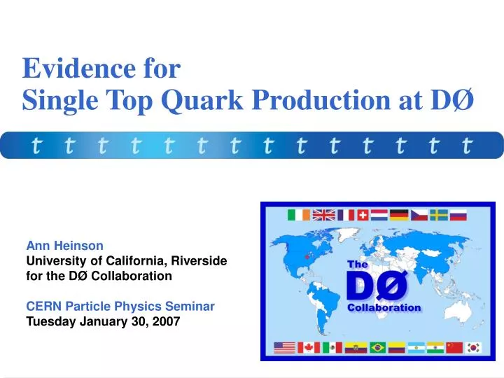
Evidence for Single Top Quark Production at DØ. Ann Heinson University of California, Riverside for the DØ Collaboration CERN Particle Physics Seminar Tuesday January 30, 2007. Top Quarks. t. top. Spin 1/2 fermion, charge +2/3 Weak-isospin partner of the bottom quark

E N D
Evidence forSingle Top Quark Production at DØ Ann Heinson University of California, Riverside for the DØ Collaboration CERN Particle Physics Seminar Tuesday January 30, 2007
Top Quarks t top • Spin 1/2 fermion, charge +2/3 • Weak-isospin partner of the bottom quark • ~40x heavier than its partner • Mtop = 171.4 ± 2.1 GeV • Heaviest known fundamental particle [GeV] 200 150 100 50 0 up down strange charm bottom top • Produced mostly in tt pairs at the Tevatron • 85% qq, 15% gg • Cross section = 6.8 ± 0.6 pb at NNLO • Measurements consistent with this value
The DØ Experiment • Top quarks observed by DØ and CDF in 1995 with ~50 pb–1 of data Fermilab Tevatron • Still the only place to see top • Now have 40x more data precision measurements
Dataset • DØ has 2 fb–1 on tape • Many thanks to the Fermilab accelerator division! • This analysis uses 0.9 fb–1 of data collected from 2002 to 2005
Single Top Overview s-channel: “tb” NLO = 0.88 ± 0.11 pb t-channel: “tqb” NLO = 1.98 ± 0.25 pb “tW production” NLO = 0.21 pb (Too small to see at the Tevatron) Experimental results (95% C.L.) • DØ tb < 5.0 pb (370 pb–1) • CDF tb < 3.2 pb (700 pb–1) • DØ tqb < 4.4 pb (370 pb–1) • CDF tqb < 3.1 pb (700 pb–1) • CDF tb+tqb < 2.7 pb Likelihoods(960 pb–1) tb+tqb < 2.6 pb Neural networks tb+tqb = 2.7 +1.5 pb Matrix elements (significance of 2.3 ) –1.3
Motivation • Study Wtb coupling in top production • Measure |Vtb| directly (more later) • Test unitarity of CKM matrix • Anomalous Wtb couplings • Cross sections sensitive to new physics • s-channel: resonances (heavy W boson, charged Higgs boson, Kaluza-Klein excited WKK, technipion, etc.) • t-channel: flavor-changing neutral currents (t – Z / / g – c / u couplings) • Fourth generation of quarks • Polarized top quarks – spin correlations measurable in decay products • Measure top quark partial decay width and lifetime • CP violation (same rate for top and antitop?) • Similar (but easier) search than for WH associated Higgs production • Backgrounds the same – must be able to model them successfully • Test of techniques to extract a small signal from a large background
Event Selection • One isolated electron or muon • Electron pT > 15 GeV, || < 1.1 • Muon pT > 18 GeV, || < 2.0 • Missing transverse energy • ET > 15 GeV • One b-tagged jet and at least one more jet • 2–4 jets with pT > 15 GeV, || < 3.4 • Leading jet pT > 25 GeV, || < 2.5 • Second leading jet pT > 20 GeV
Signal and Background Models • Single top quark signals modeled using SINGLETOP • By Moscow State University theorists, based on COMPHEP • Reproduces NLO kinematic distributions • PYTHIA for parton hadronization • tt pair backgrounds modeled using ALPGEN • PYTHIA for parton hadronization • Parton-jet matching algorithm used to avoid double-counting final states • Normalized to NNLO cross section • 18% uncertainty includes component for top mass • Multijet background modeled using data with a non-isolated lepton and jets • Normalized to data before b-tagging (together with W+jets background)
9 W+jets Background • W+jets background modeled using ALPGEN • PYTHIA for parton hadronization • Parton-jet matching algorithm used to avoid double-counting final states • Wbb and Wcc fractions from data to better represent higher-order effects • 30% uncertainty for differences in event kinematics and assuming equal for Wbb and Wcc • W+jets normalized to data before b-tagging (with multijet background) • Z+jets, diboson backgrounds very small, included in W+jets via normalization Ann Heinson (UC Riverside)
10 Event Yields Before b-Tagging • Signal acceptances: tb = 5.1%, tqb = 4.5% • S:B ratio for tb+tqb = 1:180 • Need to improve S:B to have a hope of seeing a signal select only events with b-jets in them W Transverse Mass Electrons Muons 2 jets 3 jets 4 jets Ann Heinson (UC Riverside)
11 b-Jet Identification • Separate b-jets from light-quark and gluon jets to reject most W+jets background • DØ uses a neural network algorithm • 7 input variables based on impact parameter and reconstructed vertex • Operating point: • b-jet efficiency 50% • c-jet efficiency 10% • light-jet effic. 0.5% Ann Heinson (UC Riverside)
Event Yields after b-Tagging • Signal acceptances: tb = (3.2 ± 0.4)%, tqb = (2.1 ± 0.3)% • Signal:background ratios for tb+tqb are 1:10 to 1:50 • Most sensitive channels have 2jets/1tag, S:B = 1:20 • Single top signal is smaller than total background uncertainty • counting events is not a sensitive enough method • use a multivariate discriminant to separate signal from background
Search Strategy Summary • Maximize the signal acceptance • Particle ID definitions set as loose as possible (i.e., highest efficiency, separate signal from backgrounds with fake leptons later) • Transverse momentum thresholds set low, pseudorapidities wide • As many decay channels used as possible – this analysis shown in red box • Channels analyzed separately since S:B and background compositions differ • Separate signal from background using multivariate techniques
12 Analysis Channels W Transverse Mass Electrons Muons 1 tag 2 tags 1 tag 2 tags 2 jets 3 jets 4 jets
Systematic Uncertainties • Uncertainties are assigned for each signal and background component in all analysis channels • Most systematic uncertainties apply only to normalization • Two sources of uncertainty also affect the shapes of distributions • jet energy scale • tag-rate functions for b-tagging MC events • Correlations between channels and sources are taken into account • Cross section uncertainties are dominated by the statistical uncertainty, the systematic contributions are all small
Final Analysis Steps • We have selected 12 independent sets of data for final analysis • Background model gives good representation of data in ~90 variables in every channel • Calculate discriminants that separate signal from background • Boosted decision trees • Matrix elements • Bayesian neural networks • Check discriminant performance using data control samples • Use ensembles of pseudo-data to test validity of methods • Calculate cross sections using binned likelihood fits of (floating) signal + (fixed) background to data
17 Measuring a Cross Section • Nbkgds = 6 (ttll, ttlj, Wbb, Wcc, Wjj, multijets), Nbins = 12 chans x 100 bins = 1,200 • Cross section obtained from peak position of Bayesian posterior probability density • Shape and normalization systematic uncertainties treated as nuisance parameters • Correlations between uncertainties are properly accounted for • Signal cross section prior is non-negative and flat Ann Heinson (UC Riverside)
18 Testing with Pseudo-Data • To verify that the calculation methods work as expected, we test them using several sets (“ensembles”) of pseudo-data • Wonderful tool to test the analyses! Like running DØ many 1,000’s of times • Select subsets of events from total pool of MC events • Randomly sample a Poisson distribution to simulate statistical fluctuations • Background yields fluctuated according to uncertainties to reproduce correlations between components from normalization • Ensembles we used: • Zero-signal ensemble, (tb+tqb) = 0 pb • SM ensemble, (tb+tqb) = 2.9 pb • “Mystery” ensembles, (tb+tqb) = ? pb • Measured Xsec ensemble, (tb+tqb) = meas • Each pseudo-dataset is like one DØ experiment with 0.9 fb–1 of “data”, up to 68,000 pseudo-datasets per ensemble Ann Heinson (UC Riverside)
19 Signal-Background Separationusing Decision Trees • Machine-learning technique, widely used in social sciences, some use in HEP • Idea: recover events that fail criteria in cut-based analyses • Start at first “node ” with “training sample” of 1/3 of all signal and background events • For each variable, find splitting value with best separation between two children (mostly signal in one, mostly background in the other) • Select variable and splitting value with best separation to produce two “branches ” with corresponding events, (F)ailed and (P)assed cut • Repeat recursively on each node • Stop when improvement stops or when too few events are left (100) • Terminal node is called a “leaf ” with purity = Nsignal/(Nsignal+Nbackground) • Run remaining 2/3 events and data through tree to derive results • Decision tree output for each event = leaf purity (closer to 0 for background, nearer 1 for signal) Ann Heinson (UC Riverside)
20 Boosting the Decision Trees • Boosting is a recently developed technique that improves any weak classifier (decision tree, neural network, etc) • Recently used with decision trees by GLAST and MiniBooNE • Boosting averages the results of many trees, dilutes the discrete nature of the output, improves the performance This analysis: • Uses the “adaptive boosting algorithm”: • Train a tree Tk • Check which events are misclassified by Tk • Derive tree weight wk • Increase weight of misclassified events • Train again to build Tk+1 • Boosted result of event i : • 20 boosting cycles • Trained 36 sets of trees: (tb+tqb, tb, tqb) x (e,) x (2,3,4 jets) x (1,2 b-tags) • Separate analyses for tb and tqb allow access to different types of new physics • Search for tb+tqb has best sensitivity to see a signal – results presented here Before boosting After boosting Ann Heinson (UC Riverside)
21 Decision Tree Variables • 49 input variables • Adding more variables does not degrade the performance • Reducing the number of variables always reduces sensitivity of the analysis • Same list of variables used for all analysis channels Most discrimination power: M(alljets) M(W,tag1) cos(tag1,lepton)btaggedtop Q(lepton) x (untag1) cos(leptonbesttop,besttopCofM) cos(leptonbtaggedtop,btaggedtopCofM) Ann Heinson (UC Riverside)
22 Decision Tree Cross Checks • Select two background-dominated samples: • “W+jets”: = 2 jets, HT(lepton, ET, alljets) < 175 GeV, =1 tag • “tt”: = 4 jets, HT (lepton, ET, alljets) > 300 GeV , =1 tag • Observe good data-background agreement “W+jets” “tt” Decision Tree Outputs Electrons Muons Ann Heinson (UC Riverside)
23 Decision Tree Verification • Use “mystery” ensembles with many different signal assumptions • Measure signal cross section using decision tree outputs • Compare measured cross sections to input ones • Observe linear relation close to unit slope Input xsec Ann Heinson (UC Riverside)
24 Signal-Background Separationusing Matrix Elements • Method pioneered by DØ for top quark mass measurement • Use the 4-vectors of all reconstructed leptons and jets • Use matrix elements of main signal and background Feynman diagrams to compute an event probability density for signal and background hypotheses • Goal: calculate a discriminant: • Define PSignal as a normalized differential cross section: • Performed in 2-jets and 3-jets channels only • No matrix element for tt so no discrimination between signal and top pairs yet • Matrix element verification with ensembles shows good linearity, unit slope, near-zero intercept Ann Heinson (UC Riverside)
25 Matrix Element MethodFeynman Diagrams 2-jet channels tb tq Wbb Wcg Wgg 3-jet channels tbg Wbbg tdb Ann Heinson (UC Riverside)
26 Matrix Element S:B Separation 2-jet channels tb discriminant tq discriminant Ann Heinson (UC Riverside)
27 Matrix Element Cross Checks • Select two background-dominated samples: • “Soft W+jets”: = 2 jets, HT(lepton, ET, alljets) < 175 GeV, =1 tag • “Hard W+jets”: = 2 jets, HT(lepton, ET, alljets) > 300 GeV, =1 tag • Observe good data-background agreement Matrix Element Outputs “Soft W+jets” “Hard W+jets” High end High end Full range Full range tb tq Ann Heinson (UC Riverside)
28 Signal-Background Separationusing Bayesian Neural Networks tqb Network output Wbb Network output • Bayesian neural networks improve on this technique: • Average over many networks weighted by the probability of each network given the training samples • Less prone to over-training • Network structure is less important – can use larger numbers of variables and hidden nodes • For this analysis: • 24 input variables (subset of 49 used by decision trees) • 40 hidden nodes, 800 training iterations • Each iteration is the average of 20 training cycles • One network for each signal (tb+tqb, tb, tqb) in each of the 12 analysis channels • Bayesian neural network verification with ensembles shows good linearity, unit slope, near-zero intercept • Neural networks use many input variables, train on signal and background samples, produce one output discriminant Ann Heinson (UC Riverside)
Statistical Analysis Before looking at the data, we want to know two things: • By how much can we expect to rule out a background-only hypothesis? • Find what fraction of the ensemble of zero-signal pseudo-datasets give a cross section at least as large as the SM value, the “expected p-value” • For a Gaussian distribution, convert p-value to give “expected signficance” • What precision should we expect for a measurement? • Set value for “data” = SM signal + background in each discriminant bin (non-integer) and measure central value and uncertainty on the “expected cross section” With the data, we want to know: • How well do we rule out the background-only hypothesis? • Use the ensemble of zero-signal pseudo-datasets and find what fraction give a cross section at least as large as the measured value, the “measured p-value” • Convert p-value to give “measured signficance” • What cross section do we measure? • Use (integer) number of data events in each bin to obtain “measured cross section” • How consistent is the measured cross section with the SM value? • Find what fraction of the ensemble of SM-signal pseudo-datasets give a cross section at least as large as the measured value to get “consistency with SM”
Expected Results Matrix Elements 3.7 % 1.8 3.0 pb Bayesian NNs 9.7 % 1.3 3.2 pb Decision Trees 1.9 % 2.1 2.7 pb Expected p-value Expected significance Expected cross section +1.6 –1.4 +2.0 –1.8 +1.8 –1.5 SM = 2.9 pb SM = 2.9 pb SM = 2.9 pb Matrix Elements Zero-signal ensemble Decision Trees Probability to rule out background-only hypothesis Zero-signal ensemble Bayesian Neural Networks Zero-signal ensemble Decision Trees “Data” = SM signal + background Expected result Matrix Elements Expected result Bayesian Neural Networks Expected result
Bayesian NN Results Bayesian Neural Networks Measured result (tb+tqb) = 5.0 ± 1.9 pb Measured p-value = 0.89 % Measured significance = 2.4 Compatibility with SM = 18% Bayesian Neural Networks Zero-signal ensemble Bayesian Neural Networks SM-signal ensemble Compatibility With SM 5.0 pb 5.0 pb Probability to rule out background-only hypothesis
Matrix Element Results Matrix Elements Measured result (tb+tqb) = 4.6 pb Measured p-value = 0.21 % Measured significance = 2.9 Compatibility with SM = 21% +1.8 –1.5 Matrix Elements Zero- signal ensemble Matrix Elements SM-signal ensemble Compatibility With SM 4.6 pb 4.6 pb Probability to rule out background-only hypothesis
Matrix Element Results Discriminant output without and with signal component (all channels combined to “visualize” excess)
Decision Tree Results Decision Trees Measured result (tb+tqb) = 4.9 ± 1.4 pb Measured p-value = 0.035 % Measured significance = 3.4 Compatibility with SM = 11% Decision Trees Zero- signal ensemble Decision Trees SM-signal ensemble Compatibility With SM 4.9 pb 4.9 pb Probability to rule out background-only hypothesis
Decision Tree Results Discriminant output (all channels combined) over the full range and a close-up on the high end
ME Event Characteristics ME Discriminant < 0.4 ME Discriminant > 0.7 Mass (lepton,ET,btagged-jet) [GeV] Mass (lepton,ET,btagged-jet) [GeV] Q(lepton) x (untagged-jet) Q(lepton) x (untagged-jet)
DT Event Characteristics DT Discriminant < 0.3 DT Discriminant > 0.65 Mass (lepton,ET,btagged-jet) [GeV] Mass (lepton,ET,btagged-jet) [GeV] W Transverse Mass [GeV] W Transverse Mass [GeV]
Correlation Between Methods Choose the 50 highest events in each discriminant and count overlapping events Electrons Muons Measure cross section in 400 pseudo-datasets of SM-signal ensemble and calculate linear correlation between each pair of results Results from the three methods are consistent with each other
39 CKM Matrix Element Vtb • Weak interaction eigenstates and mass eigenstates are not the same: there is mixing between quarks, described by CKM matrix • In the SM, top must decay to W and d, s, or b quark • Constraints on Vtdand Vts give • If there is new physics, then • No constraint on Vtb • Interactions between top quark and gauge bosons are very interesting Ann Heinson (UC Riverside)
40 Measuring |Vtb| • Use the measurement of the single top cross section to make the first direct measurement of |Vtb| • Calculate a posterior in |Vtb|2 ((tb, tqb) |Vtb|2) • General form of Wtb vertex: • Assume • SM top quark decay : • Pure V–A : = 0 • CP conservation : = = 0 • No need to assume only three quark families or CKM matrix unitarity (unlike for previous measurements using tt decays) • Measure the strength of the V–A coupling, |Vtb|, which can be > 1 Ann Heinson (UC Riverside)
41 First Direct Measurement of |Vtb| |Vtbf1L| = 1.3 ± 0.2 +0.0 –0.2 |Vtb|2 = 1.0 |Vtbf1L|2 = 1.7 +0.6 –0.5 0.68 < |Vtb| ≤ 1 at 95% C.L. (assuming f1L= 1) Ann Heinson (UC Riverside)
Summary: Evidence forSingle Top Quark Production at DØ • Challenging measurement – small signal hidden in huge complex background Much time spent on tool development (b-tagging) and background modeling • Three multivariate techniques applied to separate signal from background • Boosted decision trees give result with 3.4 significance • First direct measurement of |Vtb| • Result submitted to Physical Review Letters • Door is now open for studies of Wtb coupling and searches for new physics
Results for tb and tqb Separately Decision Trees Measured result for t-channel tqb (tqb) = 4.2 pb (tb) = 1.0 ± 0.9 pb +1.8 –1.4 Decision Trees Measured result for s-channel tb