Download
1 / 57
590 likes | 704 Views
Trend Attribution of Eurasian River Discharge to the Arctic Ocean. Hydro Group Seminar, May 5 Jennifer Adam Dennis Lettenmaier. Study Period 1930-2000. -18 -12 -6 0 6. Mean Annual Air Temperature, C. Study Domain. Indigirka. Lena. Yenisey. Ob’.

E N D
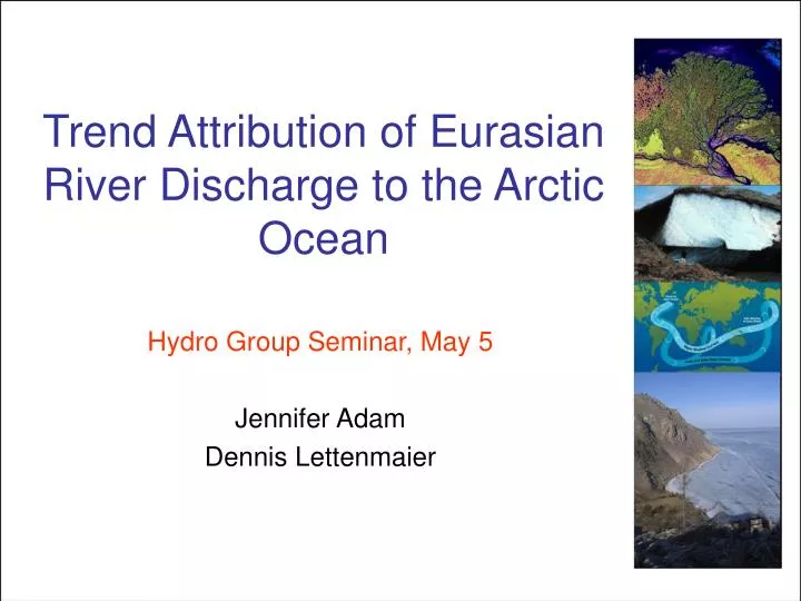
Trend Attribution of Eurasian River Discharge to the Arctic Ocean Hydro Group Seminar, May 5 Jennifer Adam Dennis Lettenmaier
Study Period 1930-2000 -18 -12 -6 0 6 Mean Annual Air Temperature, C Study Domain Indigirka Lena Yenisey Ob’ Severnaya Dvina
Annual trend for the 6 largest rivers Discharge, km3/yr Peterson et al. 2002 Discharge, km3 1950 1960 1970 1980 40 Monthly Means Ob’ GRDC 30 Discharge, m3/s 20 10 J F M A M J J A S O N D Observed Stream Flow Trends • Discharge to Arctic Ocean from six largest Eurasian rivers is increasing, 1936 to 1998: +128 km3/yr (~7% increase) • Most significant trends during the winter (low-flow) season • Purpose of study: to investigate what is causing this Winter Trend, Ob’
Climate and the Arctic • Currently experiencing system-wide change: All subsystems affected! • Rivers, temperature, precipitation, permafrost, snow, wetlands, glaciers, vegetation zonation, fire frequency, insect infestations… • Implications to global climate: • Albedo feedback • Greenhouse gas emissions/uptake • Ocean circulation feedback
Thermohaline Circulation (heat) (salt) Freshening of the Arctic Ocean deep water formation in the Northern Atlantic slowed-down or “turned-off” www.noaa.gov
Stream Flow Trend Attribution • Water Balance: Storage,S: ground water/ice, lakes, surface ice… ? ? ? • Hypothesized contributors – • Acceleration of the hydrologic cycle: P , E? • Permafrost Degradation: dS/dt, E? • Reservoir Operation: dS/dt?, E? • Other: fires, land use, wetlands, clouds, … • Published authors to date all say, “we don’t know”: McClelland et al. (2004), Berezovskaya et al. (2004), Pavelsky and Smith (2006)…
Permafrost Primer Unfrozen Frozen Frozen Unfrozen Permafrost: Coldest climates Active Layer Depth (ALD) The hydrologically active layer Seasonally Frozen Ground: Moderate to Cold climates Warming can cause the ALD to increase and/or the extent of permafrost to decrease – both affect runoff generation
Affects of Permafrost Change on Stream Flow • Seasonal effects: • Increased ALD, delay of freeze-up Increase in late fall/winter stream flow? • Annual increase via melt of excess ground ice: ice in excess of the volume of the soil pores had the soil been unfrozen * massive ice * flakes or thin layers * expanded soil pores
Continuous , 90-100% Isolated, <10% Discontinuous, 50-90% Seasonally Frozen Ground Sporadic, 10-50% Permafrost Distribution Lena: 100% permafrost (all types) Yenisey: 89% permafrost (all types) Ob’: 26% permafrost (all types) Brown et al. 1998
0.4 0.4 (+) Correlation 0.2 0.2 0.0 0.0 T/Q Correlation T/Q Correlation (-) Correlation -0.2 -0.2 -0.4 -0.4 -15 -10 -5 0 Air Temperature, C 0 5 10 15 20 Discontinuous Permafrost, % Annual Air Temperature/Stream Flow Correlation COLD: no T control on Q THRESHOLD: T control through permafrost melt WARM: T control through Evapotranspiration
Annual Precipitation/Stream Flow Correlation ΔE sensitivity to ΔP ΔQ sensitivity to ΔP “P-PET” is indicator of ΔE sensitivity to ΔP (P-PET) << 0 indicates high sensitivity, therefore ΔP contributes more towards ΔE than ΔQ, and P/Q correlation is low linear relationship for “warm” basins indicates few dS/dt effects scattered points for other basins (not shown) indicates more significant dS/dt effects
COLD: no T control on Q ΔE ~ 0 ? ΔdS/dt ~ 0 ΔP ~ ΔQ THRESHOLD: T control through permafrost melt ΔE ? ΔdS/dt < 0, according to amount of “threshold” ΔP < ΔQ WARM: T control through Evapotranspiration ΔE = f (ΔP , ΔT , P-PET) ΔdS/dt ~ 0 │ΔP │> │ΔQ │, depending on ΔT, P-PET permafrost Hypothesis Formulation
Trend Analysis • Selection of trend test: * Sensitive to seasonal differences in trend • Varying periods between 1936 and 1998 • Test for 99% significance, two-tailed • Calculate trends for precipitation, temperature, and stream flow (gauged and reconstructed (McClelland et al. 2004))
Precipitation Trends, 99% Temperature Trends, 99% Lena Yenisey Ob’ Secondary Basins C/year mm/year
Stream Flow Trends, 99% Ob’ Indigirka Lena Aldan (Lena) Lena(head) Ob’(head) Yenisey S. Dvina mm/year
Precipitation Trends (for periods with stream flow 99%) Ob’ Indigirka Lena Aldan (Lena) Lena(head) Ob’(head) Yenisey S. Dvina mm/year
Lena • Reservoir • Precipitation • Permafrost? • ET? Yenisey • Permafrost • Reservoir • Precipitation? Ob’ • Precipitation • ET • Reservoir? Aldan (Lena) • Permafrost • Precipitation? Severnaya Dvina (1)Precipitation (2)ET? Lena (head) (1)Precipitation Stream Flow/Precipitation Trends Gauged Recon. Stream Flow Trend, mm/yr Gauged Precipitation Trend, mm/yr
Reservoir filling: 1966-1970 Lena at Kusur Vilyuy at Khatyrik-Khomo Vilyuiskoe Reservoir Vilyuy at Chernyshevskiy
Q Differences: (1970-1994)-(1959-1966)(post-dam) – (pre-dam)
Modeling Application • VIC 4.1.0 r3 • Lakes • Frozen soil • Blowing snow • EASE 100 km • Calibration / Validation: • Su et al. 2005 • river discharge, snow cover extent, ice freeze-up/break-up, ALD (with problems) Su et al. 2005
Simulated Naturalized Observed Simulated Q Trend Validation Lena • VIC land surface hydrology model – complete water and energy balance • Controls handled: (1)Precipitation: YES (2)Temperature on evaporation: YES (3)Temperature on Permafrost: SOON (4) Reservoirs: NO Yenisey Annual Stream Flow, 103 m3/s Ob’
Simulated Stream Flow Trends, 99% Ob’ Indigirka Lena Aldan (Lena) Lena(head) Ob’(head) Yenisey S. Dvina mm/year
Observed Stream Flow Trends, 99% Ob’ Indigirka Lena Aldan (Lena) Lena(head) Ob’(head) Yenisey S. Dvina mm/year
Lena: X Ob’: ~ Ob’(head): ~ Irtish: S. Dvina: ~ Observed/Simulated Stream Flow Trends Gauged Recon. Observed Trend, mm/yr Gauged Simulated Trend, mm/yr
Study Period 1930-2000 -18 -12 -6 0 6 Mean Annual Air Temperature, C Study Domain Indigirka Lena Yenisey Ob’ Severnaya Dvina
ΔQ Fraction Explained by ΔP Fraction Explained by ΔE Fraction Explained by ΔdS/dt
Historical P/T Variability Historical P Variability / Climatology T Historical T Variability / Climatology P
Cherkauer finite difference algorithm • solving of thermal fluxes through soil column • infiltration/runoff response adjusted to account for effects of soil ice content • parameterization for frost spatial distribution • tracks multiple freeze/thaw layers • can use either “no flux” or “constant flux” bottom boundary current set-up: • constant flux – damping depth of 4m, Tb defined as annual ave air temperature, 15 nodes utilized • spatial frost turned on
“Noflux” On Motivation: Bottom boundary temperature no longer constrained – model is free to predict this as well as how this responds to various changes in climate, ground cover, and soil state. Necessitates deepening simulation depth to ~3x the annual damping depth (so, needs to be 10-20m) For nodes below bottom of third soil layer, total moisture derived from bottom soil moisture layer Temperature, °C Dp = 4 m, Tb(init) = -12 °C Dp = 15 m, Tb(init) = -3 °C
Tb Sensitivity to Tb(init): therefore init at zero, spin-up full 70 years at 1930’s climatology
Effect of exponential node distributions (18 nodes, 15 m) Depth Exponential Linear Time (one year)
temporal: 1800’s through 1990, but not continuous monthly data depths: 2cm, 5cm, 10cm, 15cm, 20 cm, 30 cm, 80 cm, 1.6 m, 3.2 m Depth, m Simulated versus observed soil temperatures, Ob’ station for 9/1960, linear node distribution (18 nodes, dp = 15m, tb,init = zero) Temperature, °C
Yenisey stations mean monthly biases bias varies with month and with depth Temperature, °C Month
Global Soil Moisture Database (Robock) From other datasets: • snow depth • soil temperature • air temp, precip • radiation data Two sites selected for detailed analysis – red circles
0-10 cm 0-20 cm 0-50 cm 0-100 cm
Excess Ground Ice in VIC (ice in excess of the volume of the soil pores had the soil been unfrozen) • Segregation Ice: • the first to respond to warming (i.e. usually exists in expanded soil pores – most often in clays) • Initialize model with ice-filled expanded soil pores • according to ground ice content maps • as ice thaws due to climatic warming, allow the soil pores to collapse to natural state by updating porosity (and accounting for 9% volume change from liquid to solid) • Intrusive Ice: • can be found as massive ice – often the last and slowest response to warming • add a soil layer of pure ice to VIC
Ongoing Modeling Foci • Off-line macro-scale hydrologic land surface modeling • Explore contributions to stream flow trends outside permafrost regions (Ob, S. Dvina) • Problems with permafrost simulations identified: • Needs dynamic bottom boundary temperatures (at soil damping depth) • Investigate using observed soil (and other) data • Needs incorporation of excess ground ice • Stream Flow Predictions – using downscaled GCM output
Sensitivity of Q Trend to Calibration Parameters Acknowledgements: Xiaogang Shi
Seasonal Mann-Kendall where (normally distributed, mean of zero) Calculation of Slope Estimator, B: for all pairs , and .
mm/year mm/month 300 Lena 80 40 200 3 6 9 12 0 1940 1960 1980 2000 Precipitation Data mm/year mm/month Lena 100 600 50 400 0 3 6 9 12 1940 1960 1980 2000 UW(gauge-based) Gauge-Based Reanalysis UW Data Development mm/year Lena short-term variability + long-term variability + monthly climatology Stream Flow Data Reconstructed Gauged