Spicule Family Tree

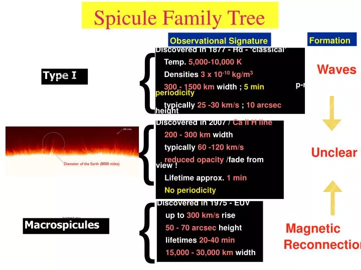
1. Spicule Family Tree Formation Observational Signature { Discovered in 1877 - Hα - ‘classical’ Temp. 5,000-10,000 K Densities 3 x 10-10 kg/m3 300 - 1500 km width ; 5 min periodicity typically25 -30 km/s ; 10 arcsec height Waves p-mode leakage Type I { Discovered in 2007/ Ca II H line 200 - 300 km width typically60 -120 km/s reduced opacity /fade from view ! Lifetime approx. 1 min No periodicity Type II Unclear reconnection ? waves ? { Discovered in 1975 - EUV up to 300 km/s rise 50 - 70 arcsec height lifetimes 20-40 min 15,000 - 30,000 km width Macrospicules Magnetic Reconnection Erupting loop Spiked Jet

2. SST/CRISP Data Scharmer et al., 2003a; 2006, 2008 Crisp (Scharmer, 2008) (1) Installation of fast 2-D spectropolarimetric imagers at the SST with a large aperture (1-m). Back -illuminated CCD cameras (sarnoff) (2) Includes a dual Fabry-Perot interferometer with fast wavelength tuning (<50 ms) which is ideally suited for observing the chromosphere. Advantage of FPI’s is that they allow for fast wavelength tuning. (3) Allows for narrow band observations at very high spectral spatial and temporal resolution. (3) All datasets are complemented with complemented with wideband images from the CRISP prefilter (FWHM 0.93 nm centered on 8542.0). There is the transmitted and reflected beam. (4) Wideband yields continuum intensity and essentially maps the photospheric revealing bright points which are concentrations of magnetic flux. (5) Atmospheric turbulence is compensated with adaptive optics (AO) (6) CRISP is mounted on the red beam of SST AO corrected light (tip tilt mirror, correlation tracker) passes throught the chopper (35 fps) and the prefilter. with part of the light being reflected to the wideband. The other part is modulated with liquid crystals producing linear combinations of the 4 stokes parameters. (4) AO + MOMFBD image restoration time sequences are of excellent quality. Diffraction limit = lambda/D 0.18 arsec. The crisp system (1024x1024) and restoration yields an image scale of 0.057 arcsec per pixel. SST/CRISP • Advance • - CRisp Imaging Spectro-Polarimeter (2008) • Dual Fabry-Pérot interferometer (FPI) • 1-m Swedish Solar Telescope (La Palma) • Line sampling between 510 - 860 nm: 36 fps • Chromosphere and Photosphere analysis in: • Red Beam (nb + wb) Blue Beam • Ca II 8542 Å (Infra-red triplet) G-Band • H-alpha 6563 Å Ca II H • Na D 5896 Å • Mg b 5172 Å • Fe I 6301 & 6302 Å • 60 x 60 arcsec FOV • 0.06 arcsec / pixel - after image restoration Co-observing: SST (CRISP) and SDO

3. Credits : T. Berger Lockheed; Movie credits – M. Carlsson ; Dave Jess/QUB

4. Image Credit : DOT SUNSPOTS Dark spots on Sun (Galileo) cooler than surroundings ~3700K. Last for several days (large ones for weeks) Sites of strong magnetic field (~3000G) Dark central umbra (strong B) Filamentary penumbra. (inhibit convection) Arise in pairs with opposite Polarity Part of the solar cycle Typical temperature of 4,000 – 4,500 Faculae typical sizes of 10,000 – 100,000 km

5. Image credit: G. Scharmer, ISP/SST

6. SST/CRISP data reduction: MOMFBD Reduction Steps MOMFBD: Destretching : algorithm removies residual image distortion left by the restoration process. destretch the image i.e creates a mask to remove the rubber sheet effect of the isoplanatic patches on the data in step 11. Flatfielding : corrrects the pixel to pixel inhomogenieties in the CCD camera.To correct the camera is illuminated with a light source and intensity variations are revealled resulting from sensitivities, dirt and fringes. (1) adaptive optics: facilitates solar imaging with significantly reduced low-order aberrations. However, due to the time scale of seeing evolution, AO only manages limited high-order corrections. (2) MOMFBD process- ing, we use simultaneously recorded wideband images as a so- called anchor channel to ensure precise alignment between the sequentially recorded CRISP narrowband images. (3) All images collected at a particular time, t, share the same realization of the random seeing phase aberrations in a method known as phase diversity (4) The passage of the wave front which distorts the atmosphere is modelled and minimized to determine the correction which is applied to all cameras. • Raw data -> Gain Corrected (flat fielding + dark current correction) • Offset calibration : Aligning Crisp-R and Crisp-T with WB pinholes to subpixel accuracy. • MOMFBD • LRE/HRE Calibration: Prefilter correction • Destretching + alignment + derotation MOMFBD van der Voort et al., 2005 • A known relation exists between the wavefronts of a set of images • Each camera (Object i) is simultaneously imaged in a number of focus diversity channels (sufficiently close in wavelength), indicated with an index k i.e. a wavelength sampling. • By exposing multiple cameras (Objects i) a set of images can be obtained for which the degradation of the images due to atmospheric distortions is identical. • The solution to the MOMFBD problem is to minimize the maximum likelihood error metric that measures the difference between the data frames and model data frames

7. Co-alignment across multiple instruments SDO ω is the angle between solar north and the optical table. φ is the azimuth. θ is the elevation. TC is the table constant. β is the tilt angle between first mirror in the telescope and solar north, i.e. a constant 14 XRT SOT SST

8. Alignment of the SST data with SDO