Download
1 / 25
250 likes | 347 Views
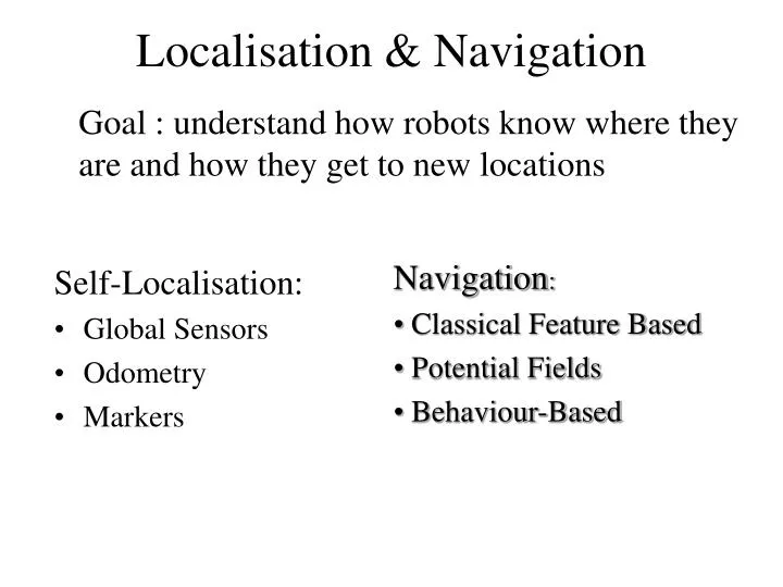
Localisation & Navigation. Goal : understand how robots know where they are and how they get to new locations. Self-Localisation: Global Sensors Odometry Markers. Navigation : Classical Feature Based Potential Fields Behaviour-Based. Global Sensors.

E N D
Localisation & Navigation Goal : understand how robots know where they are and how they get to new locations Self-Localisation: • Global Sensors • Odometry • Markers • Navigation: • Classical Feature Based • Potential Fields • Behaviour-Based
Global Sensors • Satellite Global Position Sensors (GPS) • Outdoor ok – c. 10m accuracy • Military differential GPS < 1m accuracy • Near buildings – too many reflections • Indoors: • Satellite signal not received • Local transmitters usable Buried cables give route and position
Odometry • Odometry: position measurement by distance • travelled • Know current position • Know how much wheels rotate • (e.g. current * time) • New position = old position + commanded • motion • But: • motors inaccurate -> use shaft encoders • wheels slip on surface -> also need some • feature tracking
Khepera Odometry Wheel Geometry: Non-Holonomic – must rotate about central vertical axis by wheel rotation counts L = -R
Computing Khepara position • N=600 encoder pulses/full wheel rotation • L & R encoder pulses commanded (or speed & • time) • Wheel radius • Left/right wheel travel: & • Wheel separation d
Khepera Position II If Khepera rotating: If not rotating:
Khepera Inverse Kinematics Assume smooth path Compute from change in bearing Compute h from change in position Compute Compute left & right wheel pulse increments (L & R)
Navigating With Beacons Dead reckoning: wheel slip means increasing error Periodically observe markers to recalculate position Classical style: sense, compute, act Beacons: easily identifiable features: IR LEDs special markers, bar codes
2D Beacon Observation Observe direction to 3 beacons Beacons have known position Angle and between pairs of beacons Locate self by triangulation Need lots of beacons
Beacons with range Assume can measure distances (u,v) to 2 beacons (A,B) as well as bearing (e.g. with a range sensor)
Beacons cont. • Need: • Lots of beacons • Map of beacon location • Easily identifiable beacons • Common alternative: • Use existing scene features: doorways, corners
Navigation I Planning how to get to destination Keeping track of current position • Classical robotics approach • Sense: localisation (previous) • Plan: path planning (now) • Act: move (kinematics) • Repeat 1-3 until at goal
Path Planning I Get route from current point to destination that avoids obstacles Assume a world map, with observable features in known positions (e.g. corners, doors, walls)
Avoiding Obstacles Simplest approach for convex robots is to enlarge environment by size of robot
Route Planning I • Graph search: • Nodes: floor regions + centre of mass • Arcs: connectivity & straight line distance • between lines of sight Here graph trivial. Normally use Dijkstra’s Algorithm for shortest route
Route Planning II More realistic graph
Route Planning – Potential Fields • Give a scene free space map, compute 2 fields: • F(x,y): distance from nearest obstacle • (eg. corridor wall) • G(x,y): distance from goal position
Potential Fields II Define H(x,y)=F(x,y)-k*G(x,y) Move in direction of maximum gradient: : Force vector from walls : Force vector towards goal Avoids walls while moving towards goal Avoids explicit path planning Need only compute F,G near current position Local minina possible: stuck
Mars Rovers 2 Rovers: Spirit & Opportunity Opportunity: 1350 Sols travel, 11.5 km (design: 90 Sols) Humans: route goals Robot: route following, obstacle detection, power and motor management Victoria crater (0.8 km diameter) route from Sol 860-952
Reactive Navigation I Classical Robot Control Paradigm
Reactive Navigation II Reactive: responds immediately to sensor data MIT’s Rodney Brooks Subsumption Architecture Hierarchy of parallel behaviours Upper depend on, but also override lower ones
Reactive Navigation III Run video
Reactive Navigation IV Genghis’s leg Augmented (with timers) Finite State Machine
Localisation & Navigation Summary • Global features/beacons allow direct position • feedback • 2. Odometry: position based on estimated motion • 3. Path planning using symbolic (graph) or • numerical (potential fields) • 4. Reactive methods respond to world rather than • model it