Download
1 / 47
470 likes | 589 Views
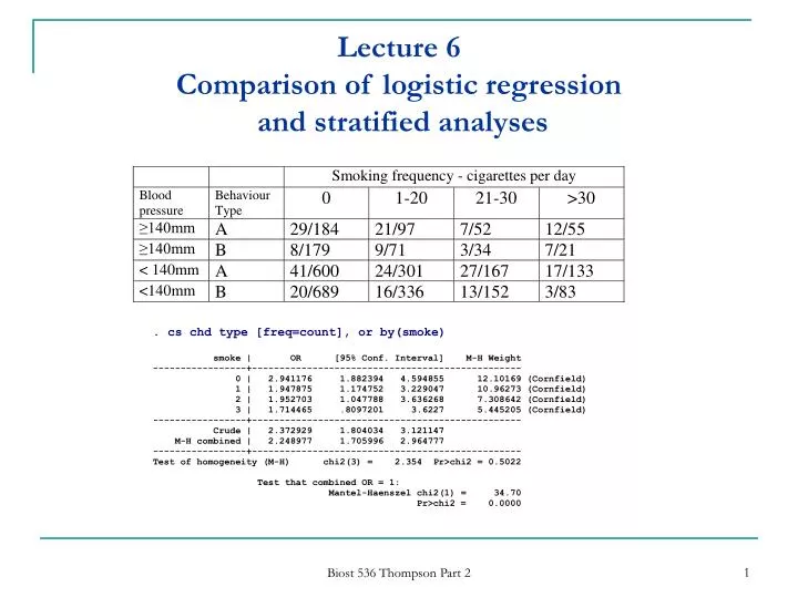
Lecture 6 Comparison of logistic regression and stratified analyses. . lincom _Itype_1+ _ItypXsmo_1_1 ( 1) _Itype_1 + _ItypXsmo_1_1 = 0 ------------------------------------------------------------------------------

E N D
Lecture 6Comparison of logistic regression and stratified analyses Biost 536 Thompson Part 2
. lincom _Itype_1+ _ItypXsmo_1_1 ( 1) _Itype_1 + _ItypXsmo_1_1 = 0 ------------------------------------------------------------------------------ chd | Odds Ratio Std. Err. z P>|z| [95% Conf. Interval] -------------+---------------------------------------------------------------- (1) | 1.947875 .5067205 2.56 0.010 1.169848 3.243343 ------------------------------------------------------------------------------ . lincom _Itype_1+ _ItypXsmo_1_2 ( 1) _Itype_1 + _ItypXsmo_1_2 = 0 ------------------------------------------------------------------------------ chd | Odds Ratio Std. Err. z P>|z| [95% Conf. Interval] -------------+---------------------------------------------------------------- (1) | 1.952703 .6272995 2.08 0.037 1.040376 3.665067 ------------------------------------------------------------------------------ . lincom _Itype_1+ _ItypXsmo_1_3 ( 1) _Itype_1 + _ItypXsmo_1_3 = 0 ------------------------------------------------------------------------------ chd | Odds Ratio Std. Err. z P>|z| [95% Conf. Interval] -------------+---------------------------------------------------------------- (1) | 1.714465 .6671239 1.39 0.166 .7996751 3.675732 ------------------------------------------------------------------------------ Biost 536 Thompson Part 2
What null hypothesis is this LRT assessing? Biost 536 Thompson Part 2
Some Stata language for recoding variables: Categorical variable “age” coded 1,2,3,4,5,6 . generate agegp=recode(age,2,4,6) . * All obsns with age <= 2 have agegp=2, all with age >2 and <=4 . * have agegp=4 and all with age > 4 and <=6 have agegp=6 . * Change the coding to 1,2,3 . recode agegp 2=1 4=2 6=3 .table age ----------+----------- Age in | years | Freq. ----------+----------- 25-34 | 116 35-44 | 199 45-54 | 213 55-64 | 242 65-74 | 161 75+ | 44 ----------+----------- Biost 536 Thompson Part 2
. drop agegp . gen agegp=recode(age,2,4) . table agegp -------+----------- agegp | Freq. -------+----------- 2 | 315 4 | 660 -------+----------- . * All observations that are not <= a number in the list are given the last value in the list . drop agegp . gen agegp=1+(age>2)+(age>4) . table agegp ----------+----------- agegp | Freq. ----------+----------- 1 | 315 2 | 455 3 | 205 ----------+----------- Biost 536 Thompson Part 2
Effect of linear transformations of covariates Biost 536 Thompson Part 2
Dose response models Consider the role of alcohol in the esophageal cancer study, with age as a potential confounder (alcohol consumption 0-39, 40-79, 80-119, 120+ g/day; age 25-34, 35-44, 45-54, 55-64,65-74,75+) . 1. Dummy variable coding • What is the interpretation of β1,β2, β3 ? • How do we state the assumption of no association between alcohol consumption and disease risk in terms of model parameters? • What does H0 : β2 =0 mean? Biost 536 Thompson Part 2
Dose response models • What is the interpretation of β1? • How would you put H0 : β1=0 into words? Biost 536 Thompson Part 2
Dose response models Comparing dummy variable and grouped linear dose-response The two models are nested. The dummy variable model is a reparameterization of a model that adds terms to the grouped linear model. Biost 536 Thompson Part 2
Dose response models Consider the following coding in a model where smoking status (cigs/day) is a risk factor: • What is the interpretation of H0 : β1=0? • What is the interpretation of H0 : β2=0? Note: the grouped linear model for smoking is nested in this model, comparing the two models provides a test of H0: β1 = β2 Biost 536 Thompson Part 2
Stata analysis Biost 536 Thompson Part 2
Fit a model without alcohol: Biost 536 Thompson Part 2
Test significance of dummy variable model ORs Compare dummy variable and grouped linear models Create plots of the fitted values for grouped linear and dummy variable models: Biost 536 Thompson Part 2
Example from the Framingham study Assume that cholesterol is the risk factor of interest for CHD and that age and sex are regarded as possible confounders Coding: Sex: Male=0 Female=1 Age: 30-49 yrs=0 50-62 yrs=1 Chol=0 <190 mg/100ml 1 190-219 mg / 100ml 2 220-249 mg /100ml 3 250+ mg/ 100ml . infile sex age chol case count using "p:\536\framingham.txt" . gen sa=sex*age . logistic case sex age sa [freq=count] Logistic regression Number of obs = 4856 LR chi2(3) = 223.78 Prob > chi2 = 0.0000 Log likelihood = -1238.1973 Pseudo R2 = 0.0829 ------------------------------------------------------------------------------ case | Odds Ratio Std. Err. z P>|z| [95% Conf. Interval] -------------+---------------------------------------------------------------- sex | .2343622 .0436654 -7.79 0.000 .1626654 .3376601 age | 2.708977 .3646438 7.40 0.000 2.080792 3.526809 sa | 2.170123 .5172673 3.25 0.001 1.36017 3.462386 ------------------------------------------------------------------------------ . est store A Biost 536 Thompson Part 2
. logistic case sex age [freq=count] Logistic regression Number of obs = 4856 LR chi2(2) = 212.83 Prob > chi2 = 0.0000 Log likelihood = -1243.6693 Pseudo R2 = 0.0788 ------------------------------------------------------------------------------ case | Odds Ratio Std. Err. z P>|z| [95% Conf. Interval] -------------+---------------------------------------------------------------- sex | .3673749 .041778 -8.81 0.000 .2939751 .4591012 age | 3.516703 .3839374 11.52 0.000 2.839262 4.35578 ------------------------------------------------------------------------------ . est store B . lrtest A B Likelihood-ratio test LR chi2(1) = 10.94 (Assumption: B nested in A) Prob > chi2 = 0.0009 Now introduce cholesterol as a dummy variable, without and then with confounder adjustment. . xi: logistic case i.chol [freq=count] i.chol _Ichol_0-3 (naturally coded; _Ichol_0 omitted) Logistic regression Number of obs = 4856 LR chi2(3) = 85.86 Prob > chi2 = 0.0000 Log likelihood = -1307.1541 Pseudo R2 = 0.0318 ------------------------------------------------------------------------------ case | Odds Ratio Std. Err. z P>|z| [95% Conf. Interval] -------------+---------------------------------------------------------------- _Ichol_1 | 1.408998 .2849726 1.70 0.090 .9478795 2.094438 _Ichol_2 | 2.361255 .446123 4.55 0.000 1.630502 3.419514 _Ichol_3 | 3.811035 .6825005 7.47 0.000 2.682905 5.413532 ------------------------------------------------------------------------------ Biost 536 Thompson Part 2
. xi: logistic case i.chol sex age sa [freq=count] i.chol _Ichol_0-3 (naturally coded; _Ichol_0 omitted) Logistic regression Number of obs = 4856 LR chi2(6) = 278.82 Prob > chi2 = 0.0000 Log likelihood = -1210.675 Pseudo R2 = 0.1033 ------------------------------------------------------------------------------ case | Odds Ratio Std. Err. z P>|z| [95% Conf. Interval] -------------+---------------------------------------------------------------- _Ichol_1 | 1.265023 .2604385 1.14 0.253 .8449991 1.89383 _Ichol_2 | 1.959199 .3786927 3.48 0.001 1.341375 2.861587 _Ichol_3 | 3.039625 .5653248 5.98 0.000 2.111102 4.376539 sex | .2504792 .0468737 -7.40 0.000 .1735726 .3614615 age | 2.649839 .360558 7.16 0.000 2.029543 3.459718 sa | 1.6341 .3962956 2.02 0.043 1.015894 2.628504 ------------------------------------------------------------------------------ . est store B . lrtest B A Likelihood-ratio test LR chi2(3) = 55.04 (Assumption: A nested in B) Prob > chi2 = 0.0000 Now explore the dose-response for cholesterol. Consider merging the two lower categories. . gen chol2=(chol>1)+(chol>2) Biost 536 Thompson Part 2
. xi: logistic case age sex sa i.chol2 [freq=count] i.chol2 _Ichol2_0-2 (naturally coded; _Ichol2_0 omitted) Logistic regression Number of obs = 4856 LR chi2(5) = 277.50 Prob > chi2 = 0.0000 Log likelihood = -1211.3366 Pseudo R2 = 0.1028 ------------------------------------------------------------------------------ case | Odds Ratio Std. Err. z P>|z| [95% Conf. Interval] -------------+---------------------------------------------------------------- age | 2.657913 .3615256 7.19 0.000 2.035924 3.469924 sex | .2494536 .0466714 -7.42 0.000 .172876 .3599521 sa | 1.646246 .3992246 2.06 0.040 1.023466 2.64799 _Ichol2_1 | 1.702258 .2465811 3.67 0.000 1.281517 2.261134 _Ichol2_2 | 2.638887 .3545856 7.22 0.000 2.027895 3.433968 ------------------------------------------------------------------------------ . est store C . lrtest B C Likelihood-ratio test LR chi2(1) = 1.32 (Assumption: C nested in B) Prob > chi2 = 0.2500 We might also consider a grouped linear model: . logistic case sex age sa chol [freq=count] Logistic regression Number of obs = 4856 LR chi2(4) = 278.11 Prob > chi2 = 0.0000 Log likelihood = -1211.0318 Pseudo R2 = 0.1030 ------------------------------------------------------------------------------ case | Odds Ratio Std. Err. z P>|z| [95% Conf. Interval] -------------+---------------------------------------------------------------- sex | .2510722 .046962 -7.39 0.000 .1740143 .3622532 age | 2.647062 .3599985 7.16 0.000 2.027689 3.455627 sa | 1.6385 .3971248 2.04 0.042 1.01892 2.634833 chol | 1.484784 .0821353 7.15 0.000 1.332222 1.654817 ------------------------------------------------------------------------------ Biost 536 Thompson Part 2
. est store D . lrtest B D Likelihood-ratio test LR chi2(2) = 0.71 (Assumption: D nested in B) Prob > chi2 = 0.7000 Or a grouped linear model based on 3 categories: . logistic case sex age sa chol2 [freq=count] Logistic regression Number of obs = 4856 LR chi2(4) = 277.36 Prob > chi2 = 0.0000 Log likelihood = -1211.4088 Pseudo R2 = 0.1027 ------------------------------------------------------------------------------ case | Odds Ratio Std. Err. z P>|z| [95% Conf. Interval] -------------+---------------------------------------------------------------- sex | .2488943 .0465438 -7.44 0.000 .1725196 .3590802 age | 2.656132 .3612456 7.18 0.000 2.034617 3.467503 sa | 1.648407 .3997793 2.06 0.039 1.024772 2.651562 chol2 | 1.621059 .1080207 7.25 0.000 1.422585 1.847223 ------------------------------------------------------------------------------ . est store E . lrtest C E Likelihood-ratio test LR chi2(1) = 0.14 (Assumption: E nested in C) Prob > chi2 = 0.7040 Using a grouped linear model with three cholesterol categories, we next proceed to explore possible interactions between the confounders and cholesterol. Biost 536 Thompson Part 2
. gen sc=sex*chol2 . gen ac=age*chol2 . logistic case sex age sa chol2 sc [freq=count] Logistic regression Number of obs = 4856 LR chi2(5) = 279.08 Prob > chi2 = 0.0000 Log likelihood = -1210.5474 Pseudo R2 = 0.1034 ------------------------------------------------------------------------------ case | Odds Ratio Std. Err. z P>|z| [95% Conf. Interval] -------------+---------------------------------------------------------------- sex | .2962674 .0673835 -5.35 0.000 .1897079 .4626819 age | 2.656331 .3622607 7.16 0.000 2.033285 3.470291 sa | 1.773859 .4424029 2.30 0.022 1.087998 2.892078 chol2 | 1.720257 .1388469 6.72 0.000 1.468555 2.015098 sc | .8292774 .1178365 -1.32 0.188 .627694 1.095599 ------------------------------------------------------------------------------ . est store F . lrtest E F Likelihood-ratio test LR chi2(1) = 1.72 (Assumption: E nested in F) Prob > chi2 = 0.1893 . logistic case sex age sa chol2 ac [freq=count] Logistic regression Number of obs = 4856 LR chi2(5) = 291.83 Prob > chi2 = 0.0000 Log likelihood = -1204.1695 Pseudo R2 = 0.1081 ------------------------------------------------------------------------------ case | Odds Ratio Std. Err. z P>|z| [95% Conf. Interval] -------------+---------------------------------------------------------------- sex | .254191 .0477456 -7.29 0.000 .1759042 .3673198 age | 4.490304 .8809846 7.66 0.000 3.056839 6.595975 sa | 1.799092 .4374102 2.42 0.016 1.117126 2.897374 chol2 | 2.11201 .2059725 7.67 0.000 1.744548 2.556871 ac | .6036774 .0801734 -3.80 0.000 .465327 .7831619 ------------------------------------------------------------------------------ . est store G Biost 536 Thompson Part 2
. lrtest E G Likelihood-ratio test LR chi2(1) = 14.48 (Assumption: E nested in G) Prob > chi2 = 0.0001 . lincom 2*chol2 ( 1) 2 chol2 = 0 ------------------------------------------------------------------------------ case | Odds Ratio Std. Err. z P>|z| [95% Conf. Interval] -------------+---------------------------------------------------------------- (1) | 4.460585 .8700318 7.67 0.000 3.043448 6.537589 ------------------------------------------------------------------------------ . lincom chol2+ac ( 1) chol2 + ac = 0 ------------------------------------------------------------------------------ case | Odds Ratio Std. Err. z P>|z| [95% Conf. Interval] -------------+---------------------------------------------------------------- (1) | 1.274972 .1149389 2.69 0.007 1.068476 1.521376 ------------------------------------------------------------------------------ . lincom 2*chol2+2*ac ( 1) 2 chol2 + 2 ac = 0 ------------------------------------------------------------------------------ case | Odds Ratio Std. Err. z P>|z| [95% Conf. Interval] -------------+---------------------------------------------------------------- (1) | 1.625555 .2930878 2.69 0.007 1.141642 2.314586 ------------------------------------------------------------------------------ Biost 536 Thompson Part 2
Logistic models Logit(p)=β0+β1chol2+β2sex+β3age+β4sex*age+β5chol2*age Biost 536 Thompson Part 2
2.11 4.46 2.11 1.27 1.63 Biost 536 Thompson Part 2
Dose response models 3. Continuous X Biost 536 Thompson Part 2
. logistic low lwt Logistic regression Number of obs = 189 LR chi2(1) = 5.98 Prob > chi2 = 0.0145 Log likelihood = -114.34533 Pseudo R2 = 0.0255 ------------------------------------------------------------------------------ low | Odds Ratio Std. Err. z P>|z| [95% Conf. Interval] -------------+---------------------------------------------------------------- lwt | .9860401 .0060834 -2.28 0.023 .9741886 .9980358 ------------------------------------------------------------------------------ . lincom 10*lwt, or ( 1) 10 lwt = 0 ------------------------------------------------------------------------------ low | Odds Ratio Std. Err. z P>|z| [95% Conf. Interval] -------------+---------------------------------------------------------------- (1) | .8688519 .0536044 -2.28 0.023 .7698929 .9805307 ------------------------------------------------------------------------------ . logit low lwt Logistic regression Number of obs = 189 LR chi2(1) = 5.98 Prob > chi2 = 0.0145 Log likelihood = -114.34533 Pseudo R2 = 0.0255 ------------------------------------------------------------------------------ low | Coef. Std. Err. z P>|z| [95% Conf. Interval] -------------+---------------------------------------------------------------- lwt | -.0140583 .0061696 -2.28 0.023 -.0261504 -.0019661 _cons | .9983143 .7852889 1.27 0.204 -.5408235 2.537452 ------------------------------------------------------------------------------ . . predict lp, p . est store A Biost 536 Thompson Part 2
. centile lwt, c(20,40,60,80) -- Binom. Interp. -- Variable | Obs Percentile Centile [95% Conf. Interval] ---------+------------------------------------------------------------- lwt | 189 20 107 102.8034 110 | 40 120 115 120 | 60 130 123 132 | 80 150 140 160 . gen lwtc=(lwt>107)+(lwt>120)+(lwt>130)+(lwt>150) . xi: logistic low i.lwtc i.lwtc Ilwtc_0-4 (naturally coded; Ilwtc_0 omitted) Logit estimates Number of obs = 189 LR chi2(4) = 11.04 Prob > chi2 = 0.0261 Log likelihood = -111.81371 Pseudo R2 = 0.0471 ------------------------------------------------------------------------------ low | Odds Ratio Std. Err. z P>|z| [95% Conf. Interval] ---------+-------------------------------------------------------------------- Ilwtc_1 | .3410256 .1523973 -2.407 0.016 .1420374 .818788 Ilwtc_2 | .5225 .2578529 -1.315 0.188 .1986185 1.374526 Ilwtc_3 | .2891304 .1554239 -2.308 0.021 .1008149 .8292065 Ilwtc_4 | .2293103 .1213334 -2.783 0.005 .0812893 .6468657 ------------------------------------------------------------------------------ Biost 536 Thompson Part 2
Smoothing . lowess low lwt, gen(lows) . twoway (scatter low lwt) (line lows lwt, sort lcol(red)) (line lp lwt, sort ), scheme(s1mono) legend(off) xtitle(Pre-pregnancy wt (lbs)) ytitle(Prob of low birthweight) Biost 536 Thompson Part 2
Splines Instead of a simple continuous function or a step function, fit a function that is linear / quadratic / cubic within group categories, but constrained to join "nicely" at the boundaries. • Advantages: • Individual data points have a strong influence on the shape of the curve only in the interval in which they lie • More plausible than a step function • Flexibility • Relatively easy to fit • Disadvantages: • As with step function: interval choice is subjective. • Hard to report results succinctly any way but graphically. • More parameters to be fitted --- Biost 536 Thompson Part 2
Linear spline • Divide the observed values of X into k+1 categories • Define: Biost 536 Thompson Part 2
Stata example . logit low lwt s1-s4 Logistic regression Number of obs = 189 LR chi2(5) = 9.90 Prob > chi2 = 0.0781 Log likelihood = -112.38526 Pseudo R2 = 0.0422 ------------------------------------------------------------------------------ low | Coef. Std. Err. z P>|z| [95% Conf. Interval] -------------+---------------------------------------------------------------- lwt | -.0260585 .0409074 -0.64 0.524 -.1062356 .0541185 s1 | -.055212 .081114 -0.68 0.496 -.2141925 .1037685 s2 | .1424752 .1001686 1.42 0.155 -.0538516 .338802 s3 | -.0732678 .0852176 -0.86 0.390 -.2402912 .0937556 s4 | -.0004225 .0449774 -0.01 0.993 -.0885765 .0877316 _cons | 2.493599 4.084743 0.61 0.542 -5.51235 10.49955 ------------------------------------------------------------------------------ . predict lsp, p . est store B . lrtest B A Likelihood-ratio test LR chi2(4) = 3.92 (Assumption: A nested in B) Prob > chi2 = 0.4169 Biost 536 Thompson Part 2
Alternative Stata code . mkspline l1 107 l2 120 l3 130 l4 150 l5=lwt, marginal . logit low l1-l5 Logistic regression Number of obs = 189 LR chi2(5) = 9.90 Prob > chi2 = 0.0781 Log likelihood = -112.38526 Pseudo R2 = 0.0422 ------------------------------------------------------------------------------ low | Coef. Std. Err. z P>|z| [95% Conf. Interval] -------------+---------------------------------------------------------------- l1 | -.0260585 .0409074 -0.64 0.524 -.1062356 .0541185 l2 | -.055212 .081114 -0.68 0.496 -.2141925 .1037685 l3 | .1424752 .1001686 1.42 0.155 -.0538516 .338802 l4 | -.0732678 .0852176 -0.86 0.390 -.2402912 .0937556 l5 | -.0004225 .0449774 -0.01 0.993 -.0885765 .0877316 _cons | 2.493599 4.084743 0.61 0.542 -5.51235 10.49955 ------------------------------------------------------------------------------ . est store C . lrtest C A Likelihood-ratio test LR chi2(4) = 3.92 (Assumption: A nested in B) Prob > chi2 = 0.4169 Biost 536 Thompson Part 2
Sensitivity to choice of intervals . gen t1=(lwt>100)*(lwt-100) . gen t2=(lwt>125)*(lwt-125) . gen t3=(lwt>150)*(lwt-150) . gen t4=(lwt>175)*(lwt-175) . logistic low lwt t1 t2 t3 t4 . logit low lwt t1 t2 t3 t4 Logistic regression Number of obs = 189 LR chi2(5) = 8.70 Prob > chi2 = 0.1216 Log likelihood = -112.98503 Pseudo R2 = 0.0371 ------------------------------------------------------------------------------ low | Coef. Std. Err. z P>|z| [95% Conf. Interval] -------------+---------------------------------------------------------------- lwt | -.0209016 .062629 -0.33 0.739 -.1436521 .101849 t1 | -.023866 .0785323 -0.30 0.761 -.1777865 .1300544 t2 | .065341 .0469319 1.39 0.164 -.0266438 .1573259 t3 | -.0494432 .0615913 -0.80 0.422 -.1701599 .0712735 t4 | .0204834 .0587547 0.35 0.727 -.0946738 .1356405 _cons | 1.985505 6.026281 0.33 0.742 -9.82579 13.7968 ------------------------------------------------------------------------------ . predict lsp2, p . twoway (scatter low lwt) (line lp lwt, sort lcol(red)) (line lsp lwt, sort clpat(dash) lcol(green) ) (line lsp2 lwt, sort clpat(dash_dot) lcol(blue) ), scheme(s1mono) legend(off) xtitle(Pre-pregnancy wt (lbs)) ytitle(Prob of low birthweight) Biost 536 Thompson Part 2
Cubic spline . spline low lwt, knots(107,120,130,150) regress(logit) gen(csp) . twoway (scatter low lwt) (line lp lwt, sort lcol(red)) (line lsp lwt, sort clpat(dash_dot) lcol(green)) (line csp lwt, sort clpat(dash)) , scheme(s1mono) legend(off) xtitle(Pre-pregnancy wt (lbs)) ytitle(Prob of low birthweight) Biost 536 Thompson Part 2
Sensitivity to choice of intervals . spline low lwt, n(3) regress(logistic) gen(csp2) . twoway (scatter low lwt) (line lp lwt, sort lcol(red)) (line csp2 lwt, sort clpat(dash_dot) lcol(pink)) (line csp lwt, sort clpat(dash)) , scheme(s1mono) legend(off) xtitle(Pre-pregnancy wt (lbs)) ytitle(Prob of low birthweight) Biost 536 Thompson Part 2
Fractional polynomials Royston P, Ambler G, Sauerbrei W. The use of fractional polynomials to model continuous risk variables in epidemiology. Int J Epidemiol, 1999; 28: 964-974. Royston P, Altman DG. Regression using fractional polynomials of continuous covariates: parsimonious modelling. Applied Statistics, 1994; 43: 429-467. Sauerbrei W, Royston P. Building multivariable prognostic and diagnostic models: transformation of the predictors by using fractional polynomials. J R Statist Soc A, 1999; 162: 71-94. Biost 536 Thompson Part 2
Fractional polynomials . fracpoly logistic low lwt ........ -> gen double Ilwt__1 = X^-2-.5934053858 if e(sample) -> gen double Ilwt__2 = X^-2*ln(X)-.1548424581 if e(sample) (where: X = lwt/100) Logistic regression Number of obs = 189 LR chi2(2) = 7.51 Prob > chi2 = 0.0234 Log likelihood = -113.58167 Pseudo R2 = 0.0320 ------------------------------------------------------------------------------ low | Odds Ratio Std. Err. z P>|z| [95% Conf. Interval] -------------+---------------------------------------------------------------- Ilwt__1 | 3.044759 5.104863 0.66 0.507 .1138735 81.41099 Ilwt__2 | .2034832 .9615213 -0.34 0.736 .0000193 2141.511 ------------------------------------------------------------------------------ Deviance: 227.16. Best powers of lwt among 44 models fit: -2 -2. . predict fp,p . twoway (scatter low lwt, symbol(x)) (line lp lwt, sort lcol(red))(line fp lwt, sort clpat(dash_dot) lcol(green)) (line csp lwt, sort clpat(dash)), scheme(s1mono) legend(off) xtitle(Pre-pregnancy wt (lbs)) ytitle(Prob of low birthweight) Biost 536 Thompson Part 2
. fracpoly logistic low lwt, degree(3) compare ............................................ -> gen double Ilwt__1 = X^3-2.187624479 if e(sample) -> gen double Ilwt__2 = X^3*ln(X)-.5708359916 if e(sample) -> gen double Ilwt__3 = X^3*ln(X)^2-.1489532287 if e(sample) (where: X = lwt/100) Logistic regression Number of obs = 189 LR chi2(3) = 9.32 Prob > chi2 = 0.0253 Log likelihood = -112.67397 Pseudo R2 = 0.0397 ------------------------------------------------------------------------------ low | Odds Ratio Std. Err. z P>|z| [95% Conf. Interval] -------------+---------------------------------------------------------------- Ilwt__1 | .0065153 .0166058 -1.97 0.048 .0000441 .9625743 Ilwt__2 | 46656.28 277007.2 1.81 0.070 .4122545 5.28e+09 Ilwt__3 | .0013849 .0055176 -1.65 0.099 5.63e-07 3.408812 ------------------------------------------------------------------------------ Deviance: 225.35. Best powers of lwt among 164 models fit: 3 3 3. Fractional polynomial model comparisons: --------------------------------------------------------------- lwt df Deviance Gain P(term) Powers --------------------------------------------------------------- Not in model 0 234.672 -- -- Linear 1 228.691 0.000 0.014 1 m = 1 2 227.276 1.414 0.234 -2 m = 2 4 227.163 1.527 0.945 -2 -2 m = 3 6 225.348 3.343 0.403 3 3 3 --------------------------------------------------------------- Biost 536 Thompson Part 2
Selection of variables Biost 536 Thompson Part 2
Modeling associations Biost 536 Thompson Part 2
Strategies • Fit all known confounders • Significance testing • Change of estimate rule A sensible strategy: • All variables that are logically confounders should be examined for their effects as confounders by controlling for them. • If the confounder alters the estimate of interest or its standard error to an important degree, include it in the model. • If the confounder does not appreciably alter the estimate, then include it in the model if it is: • traditional (e.g. gender or age) • statistically significant • estimates are believable • there are not too many other confounders in the model • Assess the role of exposure and possible effect modification by means of hypothesis testing. Biost 536 Thompson Part 2