Download

1 / 90
900 likes | 995 Views
Explore the fundamentals of data transmission in communication systems, including theoretical analysis, Fourier analysis, and bandwidth-limited signals. Learn about key transmission technologies used in modern networks, guided and wireless media, and practical communication systems. Discover the significance of Fourier series and bandwidth limitations in signal transmission.

E N D
The Physical Layer Chapter 2
In this chapter we will look at the lowest layer depicted in the hierarchy of Fig. 1-24. It defines the mechanical, electrical, and timing interfaces to the network. We will begin with a theoretical analysis of data transmission, only to discover that Mother (Parent?) Nature puts some limits on what can be sent over a channel. Then we will cover three kinds of transmission media: guided (copper wire and fiber optics), wireless (terrestrial radio), and satellite. This material will provide background information on the key transmission technologies used in modern networks. The remainder of the chapter will be devoted to three examples of communication systems used in practice for wide area computer networks: the (fixed) telephone system, the mobile phone system, and the cable television system. All three use fiber optics in the backbone, but they are organized differently and use different technologies for the last mile.
2.1 The Theoretical Basis for Data Communication • Fourier Analysis • Bandwidth-Limited Signals • Maximum Data Rate of a Channel
2.1 The Theoretical Basis for Data Communication Information can be transmitted on wires by varying some physical property such as voltage or current. By representing the value of this voltage or current as a single-valued function of time, f(t), we can model the behavior of the signal and analyze it mathematically. This analysis is the subject of the following sections.
2.1.1 Fourier Analysis In the early 19th century, the French mathematician Jean-Baptiste Fourier proved that any reasonably behaved periodic function, g(t) with period T can be constructed as the sum of a (possibly infinite) number of sines and cosines: (2-1) where f = 1/T is the fundamental frequency, an and bn are the sine and cosine amplitudes of the nth harmonics (terms), and c is a constant. Such a decomposition is called a Fourier series. From the Fourier series, the function can be reconstructed; that is, if the period, T, is known and the amplitudes are given, the original function of time can be found by performing the sums of Eq. (2-1). A data signal that has a finite duration (which all of them do) can be handled by just imagining that it repeats the entire pattern over and over forever (i.e., the interval from T to 2T is the same as from 0 to T, etc.).
Fourier Analysis The an amplitudes can be computed for any given g(t) by multiplying both sides of Eq. (2-1) by sin(2pkft) and then integrating from 0 to T. Since only one term of the summation survives: an. The bn summation vanishes completely. Similarly, by multiplying Eq. (2-1) by cos(2pkft) and integrating between 0 and T, we can derive bn. By just integrating both sides of the equation as it stands, we can find c. The results of performing these operations are as follows:
2.1.2 Bandwidth-Limited Signals To see what all this has to do with data communication, let us consider a specific example: the transmission of the ASCII character ''b'' encoded in an 8-bit byte. The bit pattern that is to be transmitted is 01100010. The left-hand part of Fig. 2-1(a) shows the voltage output by the transmitting computer. The Fourier analysis of this signal yields the coefficients: The root-mean-square amplitudes, , for the first few terms are shown on the right-hand side of Fig. 2-1(a). These values are of interest because their squares are proportional to the energy transmitted at the corresponding frequency.
Bandwidth-Limited Signals A binary signal and its root-mean-square Fourier amplitudes. (b) – (c) Successive approximations to the original signal.
Bandwidth-Limited Signals (d) – (e) Successive approximations to the original signal.
Bandwidth-Limited Signals • No transmission facility can transmit signals without losing some power in the process. • all transmission facilities diminish different Fourier components by different amounts, thus introducing distortion. Usually, the amplitudes are transmitted undiminished from 0 up to some frequency fc [measured in cycles/sec or Hertz (Hz)] with all frequencies above this cutoff frequency attenuated. • The range of frequencies transmitted without being strongly attenuated is called the bandwidth. In practice, the cutoff is not really sharp, so often the quoted bandwidth is from 0 to the frequency at which half the power gets through. • The bandwidth is a physical property of the transmission medium and usually depends on the construction, thickness, and length of the medium.
Bandwidth-Limited Signals Given a bit rate of b bits/sec, the time required to send 8 bits (for example) 1 bit at a time is 8/b sec, so the frequency of the first harmonic is b/8 Hz. An ordinary telephone line, often called a voice-grade line, has an artificially-introduced cutoff frequency just above 3000 Hz. This restriction means that the number of the highest harmonic passed through is roughly 3000/(b/8) or 24,000/b, (the cutoff is not sharp). For some data rates, the numbers work out as shown in Fig. 2-2. From these numbers, it is clear that trying to send at 9600 bps over a voice-grade telephone line will transform Fig. 2-1(a) into something looking like Fig. 2-1(c), making accurate reception of the original binary bit stream tricky. It should be obvious that at data rates much higher than 38.4 kbps, there is no hope at all for binary signals, even if the transmission facility is completely noiseless. In other words, limiting the bandwidth limits the data rate, even for perfect channels. However, sophisticated coding schemes that make use of several voltage levels do exist and can achieve higher data rates.
Bandwidth-Limited Signals Fig.2-2 Relation between data rate and harmonics.
2.1.3 The Maximum Data Rate of a Channel • Nyquist's theorem If an arbitrary signal has been run through a low-pass filter of bandwidth H, the filtered signal can be completely reconstructed by making only 2H (exact) samples per second. If the signal consists of V discrete levels, Nyquist's theorem states: maximum date rate=2Hlog2V bits/sec • Shannon'stheorem the maximum data rate of a noisy channel whose bandwidth is H Hz, and whose signal-to-noise ratio is S/N, is given by maximum date rate=Hlog2(1+S/N )bits/sec S/N:ratio of the signal power to the noise power, called the signal-to-noise ratio. Usually, the ratio itself is not quoted; instead, the quantity 10 log10 S/N is given, called decibels (dB).
2.2 Guided Transmission Data • Magnetic Media • Twisted Pair • Coaxial Cable • Fiber Optics
2.2.2 Twisted Pair One of the oldest and still most common transmission media is twisted pair. A twisted pair consists of two insulated copper wires, typically about 1 mm thick. Twisting is done because two parallel wires constitute a fine antenna. When the wires are twisted, the waves from different twists cancel out, so the wire radiates less effectively. The most common application of the twisted pair is the telephone system. Due to their adequate performance and low cost, twisted pairs are widely used and are likely to remain so for years to come. Twisted pairs can be used for transmitting either analog or digital signals. Twisted pair cabling comes in several varieties, two of which are important for computer networks. They are category 3 twisted pairs and category 5 twisted pairs. All of these wiring types are often referred to as UTP (Unshielded Twisted Pair), to contrast them with the bulky, expensive, shielded twisted pair cables IBM introduced in the early 1980s, but which have not proven popular outside of IBM installations.
Twisted Pair Fig.2-3 (a) Category 3 UTP. (b) Category 5 UTP.
2.2.3Coaxial Cable Another common transmission medium is the coaxial cable. It has better shielding than twisted pairs, so it can span longer distances at higher speeds. Two kinds of coaxial cable are widely used. One kind, 50-ohm cable, is commonly used when it is intended for digital transmission from the start. The other kind, 75-ohm cable, is commonly used for analog transmission and cable television but is becoming more important with the advent of Internet over cable. The construction and shielding of the coaxial cable give it a good combination of high bandwidth and excellent noise immunity. The bandwidth possible depends on the cable quality, length, and signal-to-noise ratio of the data signal. Modern cables have a bandwidth of close to 1 GHz. Coaxial cables used to be widely used within the telephone system for long-distance lines but have now largely been replaced by fiber optics on long-haul routes. Coax is still widely used for cable television and metropolitan area networks, however.
Coaxial Cable Fig.2-4 A coaxial cable.
2.2.4 Fiber Optics An optical transmission system has three key components: the light source, the transmission medium, and the detector. Conventionally, a pulse of light indicates a 1 bit and the absence of light indicates a 0 bit. The transmission medium is an ultra-thin fiber of glass. The detector generates an electrical pulse when light falls on it. By attaching a light source to one end of an optical fiber and a detector to the other, we have a unidirectional data transmission system that accepts an electrical signal, converts and transmits it by light pulses, and then reconverts the output to an electrical signal at the receiving end. When a light ray passes from one medium to another, for example, from fused silica to air, the ray is refracted (bent) at the silica/air boundary, as shown in Fig. 2-5(a). Here we see a light ray incident on the boundary at an angle a1 emerging at an angle b1. The amount of refraction depends on the properties of the two media (in particular, their indices of refraction). For angles of incidence above a certain critical value, the light is refracted back into the silica; none of it escapes into the air. Thus, a light ray incident at or above the critical angle is trapped inside the fiber, as shown in Fig. 2-5(b), and can propagate for many kilometers with virtually no loss.
Fiber Optics Fig.2-5 (a) Three examples of a light ray from inside a silica fiber impinging on the air/silica boundary at different angles. (b) Light trapped by total internal reflection.
Multimode Fibers and single-mode fibers The sketch of Fig. 2-5(b) shows only one trapped ray, but since any light ray incident on the boundary above the critical angle will be reflected internally, many different rays will be bouncing around at different angles. Each ray is said to have a different mode, so a fiber having this property is called a multimode fiber. However, if the fiber's diameter is reduced to a few wavelengths of light, the fiber acts like a wave guide, and the light can propagate only in a straight line, without bouncing, yielding a single-mode fiber. Single-mode fibers are more expensive but are widely used for longer distances. Currently available single-mode fibers can transmit data at 50 Gbps for 100 km without amplification. Even higher data rates have been achieved in the laboratory for shorter distances.
Transmission of Light through Fiber Transmitted power Attenuation in decibels=10log10 recieved power The attenuation of light through glass depends on the wavelength of the light (as well as on some physical properties of the glass). For the kind of glass used in fibers, the attenuation is shown in Fig. 2-6 in decibels per linear kilometer of fiber. The attenuation in decibels is given by the formula Three wavelength bands are used for optical communication. They are centered at 0.85, 1.30, and 1.55 microns, respectively. The last two have good attenuation properties (less than 5 percent loss per kilometer). The 0.85 micron band has higher attenuation, but at that wavelength the lasers and electronics can be made from the same material (gallium arsenide). All three bands are 25,000 to 30,000 GHz wide.
Transmission of Light through Fiber Fig.2-6 Attenuation of light through fiber in the infrared region.
Fiber Cables Fiber optic cables are similar to coax, except without the braid. Figure 2-7(a) shows a single fiber viewed from the side. At the center is the glass core through which the light propagates. In multimode fibers, the core is typically 50 microns in diameter, about the thickness of a human hair. In single-mode fibers, the core is 8 to 10 microns. Fig.2-7 (a) Side view of a single fiber. (b) End view of a sheath with three fibers.
Two kinds of light sources Two kinds of light sources are typically used to do the signaling, LEDs (Light Emitting Diodes) and semiconductor lasers. They have different properties, as shown in Fig. 2-8. Fig.2-8 A comparison of semiconductor diodes and LEDs as light sources.
2.3 Wireless Transmission • The Electromagnetic Spectrum • Radio Transmission • Microwave Transmission • Infrared and Millimeter Waves • Lightwave Transmission
2.3.1 The Electromagnetic Spectrum When electrons move, they create electromagnetic waves that can propagate through space (even in a vacuum). These waves were predicted by the British physicist James Clerk Maxwell in 1865 and first observed by the German physicist Heinrich Hertz in 1887. The number of oscillations per second of a wave is called its frequency, f, and is measured in Hz. The distance between two consecutive maxima (or minima) is called the wavelength, which is universally designated by the Greek letter l (lambda). When an antenna of the appropriate size is attached to an electrical circuit, the electromagnetic waves can be broadcast efficiently and received by a receiver some distance away. All wireless communication is based on this principle. In vacuum, all electromagnetic waves travel at the same speed, no matter what their frequency. This speed, usually called the speed of light, c, is approximately 3 x 10⁸ m/sec. In copper or fiber the speed slows to about 2/3 of this value and becomes slightly frequency dependent. The speed of light is the ultimate speed limit. No object or signal can ever move faster than it. The fundamental relation between f, l, and c (in vacuum) is f x l = c (2-2)
The Electromagnetic Spectrum df c cΔλ = Δf= d l l2 l2 The electromagnetic spectrum is shown in Fig. 2-11. The radio, microwave, infrared, and visible light portions of the spectrum can all be used for transmitting information by modulating the amplitude, frequency, or phase of the waves. Ultraviolet light, X-rays, and gamma rays would be even better, due to their higher frequencies, but they are hard to produce and modulate, do not propagate well through buildings, and are dangerous to living things. The bands listed at the bottom of Fig. 2-11 are the official ITU names and are based on the wavelengths, so the LF band goes from 1 km to 10 km (approximately 30 kHz to 300 kHz). The terms LF, MF, and HF refer to low, medium, and high frequency, respectively. Clearly, when the names were assigned, nobody expected to go above 10 MHz, so the higher bands were later named the Very, Ultra, Super, Extremely, and Tremendously High Frequency bands. Beyond that there are no names, but Incredibly, Astonishingly, and Prodigiously high frequency (IHF, AHF, and PHF) would sound nice. If we solve Eq. (2-2) for f and differentiate with respect to l, we get
The Electromagnetic Spectrum Fig.2-11 The electromagnetic spectrum and its uses for communication.
2.2.3 Radio Transmission Radio waves are easy to generate, can travel long distances, and can penetrate buildings easily, so they are widely used for communication, both indoors and outdoors. Radio waves also are omnidirectional, meaning that they travel in all directions from the source, so the transmitter and receiver do not have to be carefully aligned physically. The properties of radio waves are frequency dependent. At low frequencies, radio waves pass through obstacles well, but the power falls off sharply with distance from the source, roughly as 1/r2 in air. At high frequencies, radio waves tend to travel in straight lines and bounce off obstacles. They are also absorbed by rain. At all frequencies, radio waves are subject to interference from motors and other electrical equipment.Due to radio's ability to travel long distances, interference between users is a problem. For this reason, all governments tightly license the use of radio transmitters
Radio Transmission Fig.2-12 (a) In the VLF, LF, and MF bands, radio waves follow the curvature of the earth. (b) In the HF band, they bounce off the ionosphere.
2.3.3 Microwave Transmission Above 100 MHz, the waves travel in nearly straight lines and can therefore be narrowly focused. The transmitting and receiving antennas must be accurately aligned with each other. In addition, this directionality allows multiple transmitters lined up in a row to communicate with multiple receivers in a row without interference, provided some minimum spacing rules are observed. Before fiber optics, for decades these microwaves formed the heart of the long-distance telephone transmission system. Since the microwaves travel in a straight line, repeaters are needed periodically. Unlike radio waves at lower frequencies, microwaves do not pass through buildings well. In addition, even though the beam may be well focused at the transmitter, there is still some divergence in space. Some waves may be refracted off low-lying atmospheric layers and may take slightly longer to arrive than the direct waves. The delayed waves may arrive out of phase with the direct wave and thus cancel the signal. This effect is called multipath fading and is often a serious problem.
The ISM bands To prevent total chaos, there are national and international agreements about who gets to use which frequencies. Worldwide, an agency of ITU-R tries to coordinate this allocation so devices that work in multiple countries can be manufactured. Anyone who want to use some frequencies must be licensed by national and international organization. Most governments have set aside some frequency bands, called the ISM (Industrial, Scientific, Medical) bands for unlicensed usage. To minimize interference between these uncoordinated devices, all devices in the ISM bands use spread spectrum techniques. Fig.2-13 The ISM bands in the United States.
2.3.5 Lightwave Transmission Lightwave transmission is an unguided optical signaling transmission. An application is to connect the LANs in two buildings via lasers mounted on their rooftops. Coherent optical signaling using lasers is inherently unidirectional, so each building needs its own laser and its own photodetector. This scheme offers very high bandwidth and very low cost. It is also relatively easy to install and, unlike microwave, does not require an license. A disadvantage is that laser beams cannot penetrate rain or thick fog, but they normally work well on sunny days.
2.4 Communication Satellites A communication satellite can be thought of as a big microwave repeater in the sky. It contains several transponders, each of which listens to some portion of the spectrum, amplifies the incoming signal, and then rebroadcasts it at another frequency to avoid interference with the incoming signal. The downward beams can be broad, covering a substantial fraction of the earth's surface, or narrow, covering an area only hundreds of kilometers in diameter. According to Kepler's law, the orbital period of a satellite varies as the radius of the orbit to the 3/2 power. The higher the satellite, the longer the period. Near the surface of the earth, the period is about 90 minutes. Consequently, low-orbit satellites pass out of view fairly quickly, so many of them are needed to provide continuous coverage. At an altitude of about 35,800 km, the period is 24 hours. At an altitude of 384,000 km, the period is about one month, as anyone who has observed the moon regularly can testify. A satellite's period is important, but it is not the only issue in determining where to place it. Another issue is the presence of the Van Allen belts, layers of highly charged particles trapped by the earth's magnetic field. Any satellite flying within them would be destroyed fairly quickly by the highly-energetic charged particles. These factors lead to three regions in which satellites can be placed safely, and respective to three type of satellites, that is, Geostationary Satellites, Medium-Earth Orbit Satellites and Low-Earth Orbit Satellites.
Communication Satellites Fig.2-15 Communication satellites and some of their properties, including altitude above the earth, round-trip delay time and number of satellites needed for global coverage.
2.5 The Public Switched Telephone System When two computers owned by the same company or organization and located close to each other need to communicate, it is often easiest just to run a cable between them. LANs work this way. However, when the distances are large or there are many computers or the cables have to pass through a public road or other public right of way, the costs of running private cables are usually prohibitive. Consequently, the network designers must rely on the existing telecommunication facilities, especially the PSTN (Public Switched Telephone Network). • Structure of the Telephone System • The Local Loop: Modems, ADSL and Wireless • Trunks and Multiplexing • Switching
2.5.1Structure of the Telephone System Fig.2-20 (a) Fully-interconnected network. (b) Centralized switch. (c) Two-level hierarchy.
Structure of the Telephone System • In summary, the telephone system consists of three major components: • Local loops (analog twisted pairs going into houses and businesses). • Trunks (digital fiber optics connecting the switching offices). • Switching offices (where calls are moved from one trunk to another). Fig.2-22 A typical circuit route for a medium-distance call.
2.5.3 The Local Loop: Modems, ADSL, and Wireless Fig.2-23 The use of both analog and digital transmissions for a computer to computer call. Conversion is done by the modems and codecs.
The Local Loop The main parts of the system are illustrated in Fig. 2-23. Here we see the local loops, the trunks, and the toll offices and end offices, both of which contain switching equipment that switches calls. Let us begin with the part that most people are familiar with: the two-wire local loop coming from a telephone company end office into houses and small businesses. The local loop is also frequently referred to as the ''last mile,'' although the length can be up to several miles. It has used analog signaling for over 100 years and is likely to continue doing so for some years to come, due to the high cost of converting to digital. Nevertheless, even in this last bastion of analog transmission, change is taking place. In this section we will study the traditional local loop and the new developments taking place here, with particular emphasis on data communication from home computers. When a computer wishes to send digital data over an analog dial-up line, the data must first be converted to analog form for transmission over the local loop. This conversion is done by a device called a modem, something we will study shortly. At the telephone company end office the data are converted to digital form for transmission over the long-haul trunks. If the other end is a computer with a modem, the reverse conversionis needed at the destination.
Attenuation, Distortion, and Noise Transmission lines suffer from three major problems: attenuation, delay distortion, and noise. Attenuation is the loss of energy as the signal propagates outward. The loss is expressed in decibels per kilometer. The amount of energy lost depends on the frequency. To see the effect of this frequency dependence, imagine a signal not as a simple waveform, but as a series of Fourier components. Each component is attenuated by a different amount, which results in a different Fourier spectrum at the receiver. To make things worse, the different Fourier components also propagate at different speeds in the wire. This speed difference leads to distortion of the signal received at the other end. Another problem is noise, which is unwanted energy from sources other than the transmitter. Thermal noise is caused by the random motion of the electrons in a wire and is unavoidable. Crosstalk is caused by inductive coupling between two wires that are close to each other. Sometimes when talking on the telephone, you can hear another conversation in the background. That is crosstalk. Finally, there is impulse noise, caused by spikes on the power line or other causes. For digital data, impulse noise can wipe out one or more bits.
Modems Due to the problems just discussed, especially the fact that both attenuation and propagation speed are frequency dependent, it is undesirable to have a wide range of frequencies in the signal. Unfortunately, the square waves used in digital signals have a wide frequency spectrum and thus are subject to strong attenuation and delay distortion. These effects make baseband (DC) signaling unsuitable except at slow speeds and over short distances. To get around the problems associated with DC signaling, especially on telephone lines, AC signaling is used. A device that converts digital signals to analog signals (or vise versa) is called a modem (for modulator-demodulator). The modem is inserted between the (digital) computer and the (analog) telephone system.
Modulation To converts digital signals to analog signals, a continuous tone in the 1000 to 2000-Hz range, called a sine wave carrier, is introduced. Its amplitude, frequency, or phase can be modulated to transmit information. In amplitude modulation, two different amplitudes are used to represent 0 and 1, respectively. In frequency modulation, also known as frequency shift keying, two (or more) different tones are used. (The term keying is also widely used in the industry as a synonym for modulation.) In the simplest form of phase modulation, the carrier wave is systematically shifted 0 or 180 degrees at uniformly spaced intervals. A better scheme is to use shifts of 45, 135, 225, or 315 degrees to transmit 2 bits of information per time interval. Figure 2-24 illustrates the three forms of modulation. In Fig. 2-24(a) one of the amplitudes is nonzero and one is zero. In Fig. 2-24(b) two frequencies are used. In Fig. 2-24(c) a phase shift is either present or absent at each bit boundary.
Basic Technology of Modulation Fig.2-24 (a) Amplitude modulation (b) Frequency modulation (c) Absolutephase modulation (d) Relative phase modulation 0 1 0 0 1 0 A binary signal ω ω (a) ω ω ω ω ω ω 2 1 2 1 2 1 (b) π 0 π π 0 π (c)) +0 +π +0 +0 +π +0 (d))
The Concepts of Bandwidth, Baud, Symbol, and Bit Rate The concepts of bandwidth, baud, symbol, and bit rate are commonly confused, so let us restate them here. The bandwidth of a medium is the range of frequencies that pass through it with minimum attenuation. It is a physical property of the medium (usually from 0 to some maximum frequency) and measured in Hz. The baud rate is the number of samples/sec made. Each sample sends one piece of information, that is, one symbol. The baud rate and symbol rate are thus the same. The modulation technique determines the number of bits/symbol. The bit rate is the amount of information sent over the channel and is equal to the number of symbols/sec times the number of bits/symbol. To go to higher and higher speeds, it is not possible to just keep increasing the sampling rate. The Nyquist theorem says that even with a perfect 3000-Hz line (which a dial-up telephone is decidedly not), there is no point in sampling faster than 6000 Hz. In practice, most modems sample 2400 times/sec and focus on getting more bits per sample. All advanced modems use a combination of modulation techniques to transmit multiple bits per baud. Often multiple amplitudes and multiple phase shifts are combined to transmit several bits/symbol.
Advanced Modems Fig.2-25 (a) QPSK. (b) QAM-16. (c) QAM-64.
Advanced Modems (b) (a) Fig.2-26 (a) V.32 for 9600 bps. (b) V32 bis for 14,400 bps.
Digital Subscriber Lines When the telephone industry finally got to 56 kbps, it patted itself on the back for a job well done. Meanwhile, the cable TV industry was offering speeds up to 10 Mbps on shared cables, and satellite companies were planning to offer upward of 50 Mbps. As Internet access became an increasingly important part of their business, the telephone companies began to realize they needed a more competitive product. Their answer was to start offering new digital services over the local loop. Services with more bandwidth than standard telephone service are sometimes called broadband, although the term really is more of a marketing concept than a specific technical concept. Initially, there were many overlapping offerings, all under the general name of xDSL (Digital Subscriber Line), for various x. Below we will discuss these but primarily focus on what is probably going to become the most popular of these services, ADSL (Asymmetric DSL). Since ADSL is still being developed and not all the standards are fully in place, some of the details given below may change in time, but the basic picture should remain valid. For more information about ADSL, see (Summers, 1999; and Vetter et al., 2000).