Download
1 / 33
340 likes | 554 Views
Synchronous Data Flow. Synchronous Data Flow E. A. Lee and D. G. Messerschmitt Proc. of the IEEE, September, 1987.

E N D
Synchronous Data Flow Synchronous Data FlowE. A. Lee and D. G. MesserschmittProc. of the IEEE, September, 1987. Joint Minimization Of Code And Data For Synchronous Dataflow ProgramsP. K. Murthy, S. S. Bhattacharyya, and E. A. LeeMemorandum No. UCB/ERL M94/93, Electronics Research Laboratory, University of California at Berkeley Presenter: Zohair Hyder Gang Zhou
Motivation • Imperative program does not often exhibit concurrency in the algorithm • Data flow model is a programming methodology which naturally breaks a task into subtasks for more efficient use of concurrent resources
Data flow principle • Any node can fire whenever input data are available • A node with no input arcs may fire at any time • Implication: concurrency • Data-driven • Nodes are free of side effects (nodes influence each other only through data passed through arcs)
Synchronous data flow • The number of tokens produced or consumed by each node is fixed a priori for each firing • Special case: homogeneous SDF (one token per arc per firing) • A delay d is implemented by initializing arc buffer with d zero samples
Precedence graph One cycle of blocked schedule for three processors Observation: pipelining results in multiprocessor schedules with higher throughput
Large grain data flow • Large grain data flow can reduce overhead associated with each node invocation • Self loops are required to store state variables • Provides hierarchical graphical descriptions of applications
Implementation architecture • A sequential processor • Isomorphic hardware mapping • Homogeneous parallel processors sharing memory without contention
Formalism: topology matrix b(n+1) = b(n) + Γ v(n)
Scheduling for single processor • Theorem 1: For a connected SDF graph with s nodes and topology matrix Γ, rank(Γ)=s-1 is a necessary condition for a PASS (periodic admissible sequential schedule) to exist. • Theorem 2: For a connected SDF graph with s nodes and topology matrix Γ with rank(Γ)=s-1, we can find a positive integer vector q≠0 such that Γq=0. • Definition: A class S algorithm is any algorithm that schedule a node if it is runnable, updates b(n) and stops only when no more nodes are runnable. • Theorem 3: For a connected SDF graph with topology matrix Γ and a positive integer vector q s.t. Γq=0, if a PASS of period p=1Tq exists, then any class S algorithm will find such a PASS.
Theorem 4: For a connected SDF graph with topology matrix Γ and a positive integer vector q s.t. Γq=0, a PASS of period p=1Tq exists if and only if a PASS of period N*p exists for any integer N. • Corollary: For a connected SDF graph with topology matrix Γ and any positive integer vector q s.t. Γq=0, a PASS of period p=1Tq exists if and only if a PASS of period r=1Tv exists for any v s.t. Γv=0.
Sequential scheduling algorithm • Solve for smallest positive integer vector s.t. Γq=0 • Form arbitrary ordered list L of all nodes in the system • For each α in L, schedule α if it is runnable, trying each node once • If each node has been schedule qαtimes, stop and declare a successful sequential schedule • If no node in L can be scheduled, indicate a deadlock • Else go to 3 and repeat
Scheduling for parallel processors • A blocked PAPS (periodic admissible parallel schedule) is a set of lists {Ψi ,i=1,…M} where M is the number of processors and Ψi is periodic schedule for processor i • A blocked PAPS must invoke each node the number of times given by q=J*p for some positive number J called blocking factor (here p is the smallest positive integer vector in the null space of Γ) • Goal of schedule: avoid deadlock and minimize iteration period (run time for one cycle of blocked schedule divided by J) • Solution: problem identical to assembly line problem in operations research, it is NP complete, but good heuristic methods exist (Hu-level-scheduling algorithm)
Class S algorithm Initialization: i=0; q(0)=0; Main body: while nodes are runnable { for each α in L { if α is runnable then { create the j = ( qα(i) + 1 )th instance of the node α; for each input arc a on α { let β be the predecessor node for arc a compute d using d = ceil( ( - j * Γa α- ba ) / Γa β); if d < 0 then let d = 0; establish precedence links with the first d instances of β; } let v(i) be a vector with zeros except a 1 in position α; let b(i+1) = b(i) + Γ v(i) let q(i+1) = q(i) + v(i); let i = i+1; } } }
Parallel scheduling: example 3 2 3 3 J=1 6 5 3 6 J=1 3 2 6 3 J=2
JOINT MINIMIZATION OF CODE AND DATA FOR SYNCHRONOUSDATAFLOW PROGRAMS- Praveen K. Murthy, Shuvra S. Bhattacharyya, and Edward A. Lee
Chain-structured SDFs Well-ordered SDFs
Acyclic SDFs Cyclic SDFs
Schedules • Assume no delays in model • q-vector, indicates frequency of actors {A, B, C, D} firings in any cycle, e.g.: [1, 2, 3, 4]T • Can have different schedules: ABBCCCDDDD = A(2B)(3C)(4D) DDCBABCCDD = (2D)CBAB(2C)(2D) ABDDBDDCCC = A2(B(2D))(3C) • Each APPEARANCE is compiled with its associated actor’s code! • Loops are compiled once.
Objectives • Code-minimization: • Use single-appearance schedules • Data-minimization: • Minimize buffer sizes needed • Assume individual buffers for each edge • Example: consider actors A and B with q = [… 2, 2 …]T • …ABAB… • …AABB… • …2(AB)…
Buffering Cost • Consider schedule: (9A)(12B)(12C)(8D) Buffering cost: 36 + 12 + 24 = 72 • Alternate single-appearance schedule: (3(3A)(4B))(4(3C)(2D)) Buffering cost: 12 + 12 + 6 = 30 • Why not use shared buffer? • Pros: Only need maximum buffering size of any arc = 36 • Cons: 1. Implementation difficult for looped schedules 2. Addition of delays to the model modifies implementation considerably
Delays • Individual edge (e) buffers simplify addition of delays (d). • Buffering cost (e) = Original cost + d • For shared buffers, if we add delays, our circular buffer will be inconsistent • Example for q = [147, 49, 28, 32, 160]T • Buffer size = 28*8 = 224 • A = 1-147 B = 148-119 C = 120-119 …
A Useful Fact • A factoring transformation on any valid schedule yields a valid schedule: (9A)(12B)(12C)(8D) => (3(3A)(4B))(4(3C)(2D)) • Buffer requirement of factored schedule <= that of original schedule
R-schedules • Definition • Definition: A schedule is fully reduced if it is completely factored (9A)(12B)(12C)(8D) => (3(3A)(4B))(4(3C)(2D)) => (9A)(4(3BC)(2D)) • Factoring can be applied recursively to subgraphs to factor out the GCD at each step. • Result can differ depending on how graph is split: • Split between B & C => (3(3A)(4B))(4(3C)(2D)) • Split between A & B => (9A)(4(3BC)(2D)) • Set of schedules obtained this way is called set of R-schedules • Larger graphs: many R-schedules! Grows as Ω(4n/n)
R-schedules Buffering Cost • For (9A)(12B)(12C)(8D) , total 5 schedules: • (3(3A)(4B)) (4(3C)(2D)) Cost: 30 • (3(3A) (4(BC))) (8D) Cost: 37 • (3((3A)(4B) (4C))) (8D) Cost: 40 • (9A) (4(3BC) (2D)) Cost: 43 • (9A) (4(3B) (3C)(2D)) Cost: 45 • Theorum: The set of R-schedules always contains a schedule that achieves the minimum buffer memory requirement over all valid single appearance schedules. • However too many R-schedules to do exhaustive search!
Dynamic Programming • Finding optimal R-schedule is an optimal paranthesization problem. • Two-actor subchains are examined, and the buffer memory requirements for these subchains are recorded. • This information is then used to determine the minimum buffer memory requirement and the location of the split that achieves this minimum for each three-actor subchain. • And so on… • Details of algorithm described in paper. • Time complexity = Θ(n3)
Dynamic Programming – Some Details Each i-j pair represents subgraph between i-th and j-th nodes • Continue for three-actor subchains, then four-actor chains… • After finding location of split for n-actor chain, do top-down traversal to get optimal R-schedule
Example: Sample Rate Conversion • Convert 44,100 to 48,000 (CD to DAT) • 44100:48000 = 3172:2551 • q = [147, 147, 98, 28, 32, 160]T • Optimal nested schedule: (7(7(3AB)(2C))(4D))(32E(5F)) Buffering cost: 264 • Flat schedule, cost: 1021 • Shared buffer, cost: 294
Example: Sample Rate Conversion (2) Some advantages of nested schedules: • Latency: Last actor in sequence doesn’t have to wait as much. • Nested schedule has 29% less latency • Less input buffering for nested schedules.
A Heuristic • Work top-down. • Introduce split at edge where least amount of data is transferred. • Least amount of data determined with GCD of q vector elements. • Continue recursively with subgraphs. • Time complexity: Worst-case: O(n2) Average case: O(n x log n) • So-so performance
Extensions to Dynamic Programming • Delays can easily be handled by modifying the cost function. • Similarly, algorithm easily extends to well-ordered SDFs. • Algorithm can extend to general acyclic SDFs: • Use a topological sort: ordering where sources occur before sinks for every edge. • For example: ABCD, ABDC, BACD, BADC • Can find optimal R-schedule for a certain topological sort.
Extensions to Dynamic Programming (2) • Difficulties for acyclic SDFs: • There may be too many topological sorts for any SDF. • For sort ABCD => (3(4A)(3(4B)C))(16D) Cost: 208 • For sort ABDC => (4(3A)(9B)(4D))(9C) Cost: 120 • Number of sorts can grow exponentially with n. • Problem of finding optimal topological sort is NP-complete. q = [12, 36, 9, 16]T
Conclusion • Single-appearance schedules minimize code size. • Can find optimal single-appearance schedules to minimize buffer size. • Dynamic programming approach can yield results for chain-structured, well-ordered, and acyclic SDFs. • Can also work for cyclic SDFs if valid single-appearance schedule exists.