Download
1 / 36
390 likes | 679 Views
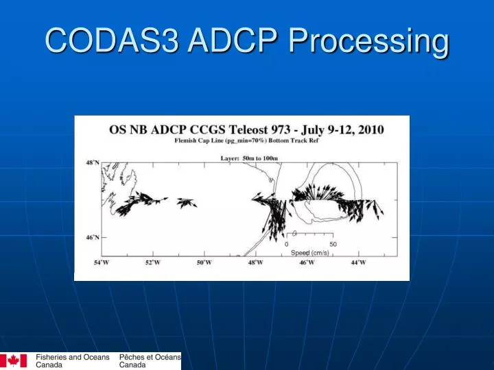
CODAS3 ADCP Processing. BPO Transect Lines. Rotation of 30°. Gridding. 1. Setup. Make ADCP tree: >>adcptree.py codas --datatype lta Setup q_py.cnt for your trip. Copy all ADCP data files into “ping” directory. Run quick_adcp.py: >>quick_adcp.py --cntfile q_py.cnt --auto

E N D
1. Setup • Make ADCP tree:>>adcptree.py codas --datatype lta • Setup q_py.cnt for your trip.
Copy all ADCP data files into “ping” directory. • Run quick_adcp.py:>>quick_adcp.py --cntfile q_py.cnt --auto • Check database to ensure data is entered:>>cd adcpdb>>showdb tel973
2. Viewing Data • From showdb, input time range into timegrid.cnt. • Run timegrid.cnt:>>timegrid timegrid.cnt
Setup adcpsect_vec.cnt for your trip. Run adcpsect_vec.cnt:>>adcpsect adcpsect_vec.cnt
Setup vector_full.cnt. • Run vector_full.cnt:>>vector vector_full.cnt • View you data.
3. Editing Data • From the “edit” directory, there are two programs to be ran: profst00.cnt and profst02.cnt. • Edit both of these according to your trip, and run them:>>profstat profst00.cnt>>profstat profst02.cnt
Edit threshld.m so that the output of profst00.cnt and profst02.cnt are entered. • Run this program within Matlab:>>threshld
The output of threshld.m will be displayed in the Matlab Command Window. • Copy these 3 values into setup.m:-D2UV_THRESHOLD-D2W_THRESHOLD-WVAR_THRESHOLD • Setup and adjust any other relevant parameters.
In the Matlab Command Window, enter one of the following two commands:>>gautoedit>>gautoedit(‘use_bt’,1) • The first command above will produce contour and vector plots using “Navigation” referencing. • The second will produce these plots using “Bottom Track” referencing. • NOTE: It may be wise to produce vector plots using both navigation and bottom track referencing to decide which is superior.
You will see a GUI similar to the one below. • From here, you can click “show now” to view your data. • There are also various pop-up menus which contain different tools for editing your data.
When you click “show now”, you will be presented with two windows. • One shows a series of contour plots, and the other has a vector plot. • Notice the bottom ringing shown in the contour plots.
When updating, ensure to click “list to disk” before you click “show next”. • Once you are finished editing, there are a series of commands you must enter to update the database. There are as follows.In Windows command prompt:>>dbupdate ../adcpdb/tel973 abottom.asc>>dbupdate ../adcpdb/tel973 abadprf.asc>>badbin ../adcpdb/tel973 abadbin.asc>>set_lgb ../adcpdb/tel973>>setflags setflags.cnt (Edit First)>>cd ../nav>>adcpsect as_nav.tmp>>refabs refabs.tmp>>smoothr smoothr.tmp
In Matlab command window:>>cd ../nav>>refsm>>cd ../edit • In Windows command prompt:putnav putnav.tmp • The database is now updated. • Repeat steps from earlier to create a vector plot, and you should see some improvements in how the data looks.
4. Contour Plots • Next, we may wish to make contour plots of the data. These plots will be done for each individual survey line. The current lines are:-Flemish Cap-Bonavista Bay-Funk Island-White Bay-Seal Island-Makkovik Bank-Beachy Island-Southeast Grand Bank-Southeast St. Pierre Bank-Southwest St. Pierre Bank
To make a contour plot, we first must slightly alter timegrid.cnt so that it only contains the time range for a particular line, say BB or FC.
Now we can run adcpsect_contour.cnt for our specified timerange. • This program must be run three times. Once for latitude, longitude, and time. • Be sure to output each variable differently ie: latfc.con, lonfc.con, timfc.con.
Once we have all three *.con files, we need to use cut.exe, paste.exe, and trans.exe to create the *.DIST file. • Run these with the following commands:>>cut –d ‘ ‘ –f 2 lonfc.con >temp>>cut –d ‘ ‘ –f 2 timfc.con >temp2>>paste temp2 temp latfc.con > tel973_fc.con>>trans tel973_fc.con tel973_fc.dist 47.000 52.833
With out *.DIST file we are now able to create contour plots. • This can be done with the use of several variations of a Python program. These are appropriately named:-Contour_U.py-Contour_U_R30.py-Contour_V.py-Contour_V_R30.py-Contour_U_ping.py-Contour_U_R30_ping.py-Contour_V_ping.py-Contour_V_R30_ping.py
5. Gridding • It is also useful to grid our data. • By putting our data into a 5m x 5km grid, we are able to smooth our data and enhance the final product.
We use the program “lateral_grid8.c” to change the *.DIST file into a *.GRID file. • This program must be compiled in CYGWIN with the following command:>>gcc –o lateral_grid8 lateral_grid8.c -lm
Once compiled, we can then run lateral_grid8 to produce the *.GRID file. • This program can be ran from command prompt with the command:>>lateral_grid8 tel973_fc.dist tel973_fc.grid 2010 • The new *.GRID file can now be contoured using the Python programs:-Contour_U_grid.py-Contour_U_R30_grid.py-Contour_V_grid.py-Contour_V_R30_grid.py