Download
1 / 79
790 likes | 822 Views
Learn how boosting algorithms convert weak learners into strong ones to classify spam emails effectively. Explore the process and types of boosting algorithms.

E N D
INTRODUCTION TO BOOSTING https://cse.iitk.ac.in/users/piyush/courses/ml_autumn16/771A_lec21_slides.pdf https://ocw.mit.edu/courses/sloan-school-of-management/15-097-prediction-machine-learning-and-statistics-spring-2012/lecture-notes/MIT15_097S12_lec10.pdf https://www.cs.toronto.edu/~hinton/csc2515/notes/lec11boo.htm http://www.ccs.neu.edu/home/vip/teach/MLcourse/4_boosting/slides/gradient_boosting.pdf http://blog.kaggle.com/2017/01/23/a-kaggle-master-explains-gradient-boosting/ https://www.analyticsvidhya.com/blog/2018/09/an-end-to-end-guide-to-understand-the-math-behind-xgboost/
DEFINITION • The term ‘Boosting’ refers to a family of algorithms which converts weak learner to strong learners. • Let’s understand this definition in detail by solving a problem of spam email identification: • How would you classify an email as SPAM or not? Like everyone else, our initial approach would be to identify ‘spam’ and ‘not spam’ emails using following criteria. If: • Email has only one image file (promotional image), It’s a SPAM • Email has only link(s), It’s a SPAM • Email body consist of sentence like “You won a prize money of $ xxxxxx”, It’s a SPAM • Email from our official domain “metu.edu.tr” , Not a SPAM • Email from known source, Not a SPAM • Above, we’ve defined multiple rules to classify an email into ‘spam’ or ‘not spam’. But, do you think these rules individually are strong enough to successfully classify an email? No. • Individually, these rules are not powerful enough to classify an email into ‘spam’ or ‘not spam’. Therefore, these rules are called as weak learner.
DEFINITION • To convert weak learner to strong learner, we’ll combine the prediction of each weak learner using methods like:• Using average/ weighted average• Considering prediction has higher vote • For example: Above, we have defined 5 weak learners. Out of these 5, 3 are voted as ‘SPAM’ and 2 are voted as ‘Not a SPAM’. In this case, by default, we’ll consider an email as SPAM because we have higher(3) vote for ‘SPAM’.
How Boosting Algorithms works? • To find weak rule, we apply base learning algorithms with a different distribution. Each time base learning algorithm is applied, it generates a new weak prediction rule. This is an iterative process. After many iterations, the boosting algorithm combines these weak rules into a single strong prediction rule. • For choosing the right distribution, here are the following steps: Step 1: The base learner takes all the distributions and assign equal weight or attention to each observation. Step 2: If there is any prediction error caused by first base learning algorithm, then we pay higher attention to observations having prediction error. Then, we apply the next base learning algorithm. Step 3: Iterate Step 2 till the limit of base learning algorithm is reached or higher accuracy is achieved. • Finally, it combines the outputs from weak learner and creates a strong learner which eventually improves the prediction power of the model. Boosting pays higher focus on examples which are misclassified or have higher errors by preceding weak rules.
Types of Boosting Algorithms • Underlying engine used for boosting algorithms can be anything. It can be decision stamp, margin-maximizing classification algorithm etc. There are many boosting algorithms which use other types of engine such as: • AdaBoost (Adaptive Boosting) • Gradient Tree Boosting • GentleBoost • LPBoost • BrownBoost • XGBoost • CatBoost • Lightgbm
AdaBoost • Box 1: You can see that we have assigned equal weights to each data point and applied a decision stump to classify them as + (plus) or – (minus). The decision stump (D1) has generated vertical line at left side to classify the data points. We see that, this vertical line has incorrectly predicted three + (plus) as – (minus). In such case, we’ll assign higher weights to these three + (plus) and apply another decision stump.
AdaBoost • Box 2: Here, you can see that the size of three incorrectly predicted + (plus) is bigger as compared to rest of the data points. In this case, the second decision stump (D2) will try to predict them correctly. Now, a vertical line (D2) at right side of this box has classified three misclassified + (plus) correctly. But again, it has caused misclassification errors. This time with three -(minus). Again, we will assign higher weight to three – (minus) and apply another decision stump.
Adaboost • Box 3: Here, three – (minus) are given higher weights. A decision stump (D3) is applied to predict these misclassified observation correctly. This time a horizontal line is generated to classify + (plus) and – (minus) based on higher weight of misclassified observation.
Adaboost • Box 4: Here, we have combined D1, D2 and D3 to form a strong prediction having complex rule as compared to individual weak learner. You can see that this algorithm has classified these observation quite well as compared to any of individual weak learner.
AdaBoost (Adaptive Boosting) • It works on similar method as discussed above. It fits a sequence of weak learners on different weighted training data. It starts by predicting original data set and gives equal weight to each observation. If prediction is incorrect using the first learner, then it gives higher weight to observation which have been predicted incorrectly. Being an iterative process, it continues to add learner(s) until a limit is reached in the number of models or accuracy. • Mostly, we use decision stamps with AdaBoost. But, we can use any machine learning algorithms as base learner if it accepts weight on training data set. We can use AdaBoost algorithms for both classification and regression problem.
Let’s try to visualize one Classification Problem • Look at the below diagram : We start with the first box. We see one vertical line which becomes our first week learner. Now in total we have 3/10 mis-classified observations. We now start giving higher weights to 3 plus mis-classified observations. Now, it becomes very important to classify them right. Hence, the vertical line towards right edge. We repeat this process and then combine each of the learner in appropriate weights.
Explaining underlying mathematics • How do we assign weight to observations? • We always start with a uniform distribution assumption. Lets call it as D1 which is 1/n for all n observations. • Step 1 . We assume an alpha(t) • Step 2: Get a weak classifier h(t) • Step 3: Update the population distribution for the next step where
Explaining underlying mathematics • Simply look at the argument in exponent. Alpha is kind of learning rate, y is the actual response ( + 1 or -1) and h(x) will be the class predicted by learner. Essentially, if learner is going wrong, the exponent becomes 1*alpha and else -1*alpha. The weight will probably increase, if the prediction went wrong the last time. • Step 4 : Use the new population distribution to again find the next learner • Step 5 : Iterate step 1 – step 4 until no hypothesis is found which can improve further. • Step 6 : Take a weighted average of the frontier using all the learners used till now. But what are the weights? Weights are simply the alpha values. Alpha is calculated as follows:
Explaining underlying mathematics • Output the final hypothesis
Gradient Boosting • In gradient boosting, it trains many models sequentially. Each new model gradually minimizes the loss function (y = ax + b + e, e needs special attention as it is an error term) of the whole system using Gradient Descent method. The learning procedure consecutively fit new models to provide a more accurate estimate of the response variable. • The principle idea behind this algorithm is to construct new base learners which can be maximally correlated with negative gradient of the loss function, associated with the whole ensemble.
Gradient Boosting • Type of Problem – You have a set of variables vectors x1 , x2 and x3. You need to predict y which is a continuous variable. • Steps of Gradient Boost algorithm Step 1 : Assume mean is the prediction of all variables. Step 2 : Calculate errors of each observation from the mean (latest prediction). Step 3 : Find the variable that can split the errors perfectly and find the value for the split. This is assumed to be the latest prediction. Step 4 : Calculate errors of each observation from the mean of both the sides of split (latest prediction). Step 5 : Repeat the step 3 and 4 till the objective function maximizes/minimizes. Step 6 : Take a weighted mean of all the classifiers to come up with the final model.
Example • Assume, you are given a previous model M to improve on. Currently you observe that the model has an accuracy of 80% (any metric). How do you go further about it? • One simple way is to build an entirely different model using new set of input variables and trying better ensemble learners. On the contrary, I have a much simpler way to suggest. It goes like this: Y = M(x) + error • What if I am able to see that error is not a white noise but have same correlation with outcome(Y) value. What if we can develop a model on this error term? Like, error = G(x) + error2
Example • Probably, you’ll see error rate will improve to a higher number, say 84%. Let’s take another step and regress against error2. error2 = H(x) + error3 • Now we combine all these together : Y = M(x) + G(x) + H(x) + error3 • This probably will have an accuracy of even more than 84%. What if I can find an optimal weights for each of the three learners, Y = alpha * M(x) + beta * G(x) + gamma * H(x) + error4
Example • If we found good weights, we probably have made even a better model. This is the underlying principle of a boosting learner. • Boosting is generally done on weak learners, which do not have a capacity to leave behind white noise. • Boosting can lead to overfitting, so we need to stop at the right point.
How to improve regression results • You are given (x1, y1), (x2, y2), …, (xn, yn), and the task is to t a model F(x) to minimize square loss. • Suppose your friend wants to help you and gives you a model F. • You check his model and find the model is good but not perfect. There are some mistakes: F(x1) = 0.8, while y1 = 0.9, and F(x2) = 1.4 while y2 = 1.3. How can you improve this model? • Rule of the game: You are not allowed to remove anything from F or change any parameter in F. You can add an additional model (regression tree) h to F, so the new prediction will be F(x) + h(x).
Simple solution: • You wish to improve the model such that F(x1) + h(x1) = y1 F(x2) + h(x2) = y2 ::: F(xn) + h(xn) = yn Or, equivalently, you wish h(x1) = y1 ̶ F(x1) h(x2) = y2 ̶ F(x2) ::: h(xn) = yn ̶ F(xn) • Can any regression tree h achieve this goal perfectly?
Maybe not.... • But some regression tree might be able to do this approximately. • How? • Just fit a regression tree h to data (x1, y1̶ F(x1)), (x2, y2̶ F(x2)), …, (xn, yn̶ F(xn)) • Congratulations, you get a better model! • yi ̶ F(xi) are residuals. These are the parts that existing model F cannot do well. • The role of h is to compensate the shortcoming of existing model F. If the new model F + h is still not satisfactory, we can add another regression tree... • We are improving the predictions of training data, but is the procedure also useful for test data? • Yes! Because we are building a model, and the model can be applied to test data as well. • How is this related to gradient descent?
How is this related to gradient descent? • For regression with square loss, residual negative gradient fit h to residual fit h to negative gradient update F based on residual update F based on negative gradient • So we are actually updating our model using gradient descent! It turns out that the concept of gradients is more general and useful than the concept of residuals. So from now on, let's stick with gradients.
Problem • Recognize the given hand written capital letter. • Multi-class classification • 26 classes. A,B,C,...,Z • Data Set • http://archive.ics.uci.edu/ml/datasets/Letter+Recognition • 20000 data points, 16 features
Feature Extraction • Feature Vector= (2, 1, 3, 1, 1, 8, 6, 6, 6, 6, 5, 9, 1, 7, 5, 10) • Label = G
Model • 26 score functions (our models): FA, FB, FC , …, FZ . • FA(x) assigns a score for class A • scores are used to calculate probabilities • predicted label = class that has the highest probability
Loss Function for each data point Step 1. turn the label yi into a (true) probability distribution Yc (xi). For example: y5=G, YA(x5) = 0, YB(x5) = 0, …, YG(x5) = 1, …, YZ(x5) = 0.
Step 2. Calculate the predicted probability distribution Pc(xi) based on the current model FA, FB, …, FZ . PA(x5) = 0.03, PB(x5) = 0.05, …, PG (x5) = 0.3, …, PZ (x5) =0.05.
Step 3. Calculate the difference between the true probability distribution and the predicted probability distribution. Here we use KL-divergence • Goal • minimize the total loss (KL-divergence) • for each data point, we wish the predicted probability distribution to match the true probability distribution as closely as possible
We achieve this goal by adjusting our models FA, FB, …, FZ . Differences • FA, FB, …, FZvs F • a matrix of parameters to optimize vs a column of parameters to optimize • a matrix of gradients vs a column of gradients
Bagging vs Boosting • No clear winner; usually depends on the data • Bagging is computationally more efficient than boosting (note that bagging can train the M models in parallel, boosting can’t) • Both reduce variance (and overfitting) by combining different models • The resulting model has higher stability as compared to the individual ones • Bagging usually can’t reduce the bias, boosting can (note that in boosting, the training error steadily decreases) • Bagging usually performs better than boosting if we don’t have a high bias and only want to reduce variance (i.e., if we are overfitting)
XGBoosting (Extreme Gradient Boosting) • Ever since its introduction in 2014, XGBoost has been lauded as the holy grail of machine learning hackathons and competitions. From predicting ad click-through rates to classifying high energy physics events, XGBoost has proved its mettle in terms of performance – and speed. • Execution Speed: Generally, XGBoost is fast. Really fast when compared to other implementations of gradient boosting. But newly introduced LightGBM is faster than XGBoosting. • Model Performance: XGBoost dominates structured or tabular datasets on classification and regression predictive modeling problems. The evidence is that it is the go-to algorithm for competition winners on the Kaggle competitive data science platform.