Download
1 / 30
320 likes | 711 Views
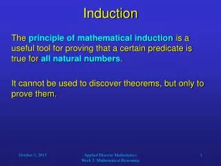
Induction. The principle of mathematical induction is a useful tool for proving that a certain predicate is true for all natural numbers . It cannot be used to discover theorems, but only to prove them. Induction.

E N D
Induction • The principle of mathematical induction is a useful tool for proving that a certain predicate is true for all natural numbers. • It cannot be used to discover theorems, but only to prove them. Applied Discrete Mathematics Week 5: Mathematical Reasoning
Induction • If we have a propositional function P(n), and we want to prove that P(n) is true for any natural number n, we do the following: • Show that P(0) is true.(basis step) • Show that if P(n) then P(n + 1) for any nN.(inductive step) • Then P(n) must be true for any nN. (conclusion) Applied Discrete Mathematics Week 5: Mathematical Reasoning
Induction • Example: • Show that n < 2n for all positive integers n. • Let P(n) be the proposition “n < 2n.” • 1. Show that P(1) is true.(basis step) • P(1) is true, because 1 < 21 = 2. Applied Discrete Mathematics Week 5: Mathematical Reasoning
Induction • 2. Show that if P(n) is true, then P(n + 1) is true.(inductive step) • Assume that n < 2n is true. • We need to show that P(n + 1) is true, i.e. • n + 1 < 2n+1 • We start from n < 2n: • n + 1 < 2n + 1 2n + 2n = 2n+1 • Therefore, if n < 2n then n + 1 < 2n+1 Applied Discrete Mathematics Week 5: Mathematical Reasoning
Induction • Then P(n) must be true for any positive integer.(conclusion) • n < 2n is true for any positive integer. • End of proof. Applied Discrete Mathematics Week 5: Mathematical Reasoning
Induction • Another Example (“Gauss”): • 1 + 2 + … + n = n (n + 1)/2 • Show that P(0) is true.(basis step) • For n = 0 we get 0 = 0. True. Applied Discrete Mathematics Week 5: Mathematical Reasoning
Induction • Show that if P(n) then P(n + 1) for any nN. (inductive step) • 1 + 2 + … + n = n (n + 1)/2 • 1 + 2 + … + n + (n + 1) = n (n + 1)/2 + (n + 1) • = (n + 1) (n/2 + 1) • = (n + 1) (n + 2)/2 • = (n + 1)((n + 1) + 1)/2 Applied Discrete Mathematics Week 5: Mathematical Reasoning
Induction • Then P(n) must be true for any nN. (conclusion) • 1 + 2 + … + n = n (n + 1)/2 is true for all nN. • End of proof. Applied Discrete Mathematics Week 5: Mathematical Reasoning
Induction • There is another proof technique that is very similar to the principle of mathematical induction. • It is called the second principle of mathematical induction. • It can be used to prove that a propositional function P(n) is true for any natural number n. Applied Discrete Mathematics Week 5: Mathematical Reasoning
Induction • The second principle of mathematical induction: • Show that P(0) is true.(basis step) • Show that if P(0) and P(1) and … and P(n),then P(n + 1) for any nN.(inductive step) • Then P(n) must be true for any nN. (conclusion) Applied Discrete Mathematics Week 5: Mathematical Reasoning
Induction • Example: • Show that every integer greater than 1 can be written as the product of primes. • Show that P(2) is true.(basis step) • 2 is the product of one prime: itself. Applied Discrete Mathematics Week 5: Mathematical Reasoning
Induction • Show that if P(2) and P(3) and … and P(n),then P(n + 1) for any nN. (inductive step) • Two possible cases: • If (n + 1) is prime, then obviously P(n + 1) is true. • If (n + 1) is composite, it can be written as the product of two integers a and b such that2 a b < n + 1. • By the induction hypothesis, both a and b can be written as the product of primes. • Therefore, n + 1 = ab can be written as the product of primes. Applied Discrete Mathematics Week 5: Mathematical Reasoning
Induction • Then P(n) must be true for any nNwith n > 1.(conclusion) • End of proof. • We have shown that every integer greater than 1 can be written as the product of primes. Applied Discrete Mathematics Week 5: Mathematical Reasoning
Recursive Definitions • Recursion is a principle closely related to mathematical induction. • In a recursive definition, an object is defined in terms of itself. • We can recursively define sequences, functions and sets. Applied Discrete Mathematics Week 5: Mathematical Reasoning
Recursively Defined Sequences • Example: • The sequence {an} of powers of 2 is given byan = 2n for n = 0, 1, 2, … . • The same sequence can also be defined recursively: • a0 = 1 • an+1 = 2an for n = 0, 1, 2, … • Obviously, induction and recursion are similar principles. Applied Discrete Mathematics Week 5: Mathematical Reasoning
Recursively Defined Functions • We can use the following method to define a function with the natural numbers as its domain: • Specify the value of the function at zero. • Give a rule for finding its value at any integer from its values at smaller integers. • Such a definition is called recursive or inductive definition. Applied Discrete Mathematics Week 5: Mathematical Reasoning
Recursively Defined Functions • Example: • f(0) = 3 • f(n + 1) = 2f(n) + 3 • f(0) = 3 • f(1) = 2f(0) + 3 = 23 + 3 = 9 • f(2) = 2f(1) + 3 = 29 + 3 = 21 • f(3) = 2f(2) + 3 = 221 + 3 = 45 • f(4) = 2f(3) + 3 = 245 + 3 = 93 Applied Discrete Mathematics Week 5: Mathematical Reasoning
Recursively Defined Functions • How can we recursively define the factorial function f(n) = n! ? • f(0) = 1 • f(n + 1) = (n + 1)f(n) • f(0) = 1 • f(1) = 1f(0) = 11 = 1 • f(2) = 2f(1) = 21 = 2 • f(3) = 3f(2) = 32 = 6 • f(4) = 4f(3) = 46 = 24 Applied Discrete Mathematics Week 5: Mathematical Reasoning
Recursively Defined Functions • A famous example: The Fibonacci numbers • f(0) = 0, f(1) = 1 • f(n) = f(n – 1) + f(n - 2) • f(0) = 0 • f(1) = 1 • f(2) = f(1) + f(0) = 1 + 0 = 1 • f(3) = f(2) + f(1) = 1 + 1 = 2 • f(4) = f(3) + f(2) = 2 + 1 = 3 • f(5) = f(4) + f(3) = 3 + 2 = 5 • f(6) = f(5) + f(4) = 5 + 3 = 8 Applied Discrete Mathematics Week 5: Mathematical Reasoning
Recursively Defined Sets • If we want to recursively define a set, we need to provide two things: • an initial set of elements, • rules for the construction of additional elements from elements in the set. • Example: Let S be recursively defined by: • 3 S • (x + y) S if (x S) and (y S) • S is the set of positive integers divisible by 3. Applied Discrete Mathematics Week 5: Mathematical Reasoning
Recursively Defined Sets • Proof: • Let A be the set of all positive integers divisible by 3. • To show that A = S, we must show that A S and S A. • Part I: To prove that A S, we must show that every positive integer divisible by 3 is in S. • We will use mathematical induction to show this. Applied Discrete Mathematics Week 5: Mathematical Reasoning
Recursively Defined Sets • Let P(n) be the statement “3n belongs to S”. • Basis step: P(1) is true, because 3 is in S. • Inductive step: To show:If P(n) is true, then P(n + 1) is true. • Assume 3n is in S. Since 3n is in S and 3 is in S, it follows from the recursive definition of S that3n + 3 = 3(n + 1) is also in S. • Conclusion of Part I: A S. Applied Discrete Mathematics Week 5: Mathematical Reasoning
Recursively Defined Sets • Part II: To show: S A. • Basis step: To show: All initial elements of S are in A. 3 is in A. True. • Inductive step: To show:(x + y) is in A whenever x and y are in A. • If x and y are both in A, it follows that 3 | x and 3 | y. As we already know, it follows that 3 | (x + y). • Conclusion of Part II: S A. • Overall conclusion: A = S. Applied Discrete Mathematics Week 5: Mathematical Reasoning
Recursively Defined Sets • Another example: • The well-formed formulas of variables, numerals and operators from {+, -, *, /, ^} are defined by: • x is a well-formed formula if x is a numeral or variable. • (f + g), (f – g), (f * g), (f / g), (f ^ g) are well-formed formulas if f and g are. Applied Discrete Mathematics Week 5: Mathematical Reasoning
Recursively Defined Sets • With this definition, we can construct formulas such as: • (x – y) • ((z / 3) – y) • ((z / 3) – (6 + 5)) • ((z / (2 * 4)) – (6 + 5)) Applied Discrete Mathematics Week 5: Mathematical Reasoning
Recursive Algorithms • An algorithm is called recursive if it solves a problem by reducing it to an instance of the same problem with smaller input. • Example I: Recursive Euclidean Algorithm • procedure gcd(a, b: nonnegative integers with a < b) • if a = 0 then gcd(a, b) := b • else gcd(a, b) := gcd(b mod a, a) Applied Discrete Mathematics Week 5: Mathematical Reasoning
Recursive Algorithms • Example II: Recursive Fibonacci Algorithm • procedure fibo(n: nonnegative integer) • if n = 0 then fibo(0) := 0 • else if n = 1 then fibo(1) := 1 • else fibo(n) := fibo(n – 1) + fibo(n – 2) Applied Discrete Mathematics Week 5: Mathematical Reasoning
f(4) f(3) f(2) f(2) f(0) f(1) f(1) f(1) f(0) Recursive Algorithms • Recursive Fibonacci Evaluation: Applied Discrete Mathematics Week 5: Mathematical Reasoning
Recursive Algorithms • procedure iterative_fibo(n: nonnegative integer) • if n = 0 then y := 0 • else • begin • x := 0 • y := 1 • for i := 1 to n-1 • begin • z := x + y • x : = y • y := z • end • end{y is the n-th Fibonacci number} Applied Discrete Mathematics Week 5: Mathematical Reasoning
Recursive Algorithms • For every recursive algorithm, there is an equivalent iterative algorithm. • Recursive algorithms are often shorter, more elegant, and easier to understand than their iterative counterparts. • However, iterative algorithms are usually more efficient in their use of space and time. Applied Discrete Mathematics Week 5: Mathematical Reasoning