Download
1 / 62
620 likes | 747 Views
Session No. DM131 New Optimizer and Query Execution Options in Adaptive Server Enterprise 12.0 . Eric Miner Development Engineer ESD Eric.Miner@sybase.com. Ian Smart Senior Evangelist ESD Ian.Smart@sybase.com. ASE 12.0 Changes. Parallel and Serial Sort/Merge Joins

E N D
Session No. DM131New Optimizer and Query Execution Options in Adaptive Server Enterprise 12.0 Eric Miner Development Engineer ESD Eric.Miner@sybase.com Ian Smart Senior Evangelist ESD Ian.Smart@sybase.com
ASE 12.0 Changes • Parallel and Serial Sort/Merge Joins • Smart Transformation of WHERE Clause Predicates • Improved Selectivity Estimation for LIKE Predicates • Join transitive closure • New Outer Join Syntax and Logic • Abstract Query Plans • Support for up to 50 tables in a join clause • Execute Immediate
Pre-optimization Join Transitive Closure ANSI Compliant Outer Joins Predicate Transformation From Query Text to Query Results Query Text • Optimization • Improved costing of “%XXX” like clauses • Abstract Query Plans • Query Execution • Sort-Merge Joins • 50 table limit • Execute Immediate Query Results
Work in progress • In ASE 11.9.x the optimizer was re-written: • sysstatistics and systabstats replaced distribution pages and provided a much greater level of detail on data distribution across the table • In the next release of ASE, the replacement for the query execution engine will be fully implemented • ASE 12.0 contains: • first phase of the replacement of the query execution engine - providing new query execution possibilities • increased intelligence in pre-optimization processing of queries
What do the icon’s mean?? • New method of calculating costs in when generating the query plan • Typically due to additional information being made available from pre-optimization processing of the query • Performance enhancement • Due to new query execution options that process the data more efficiently • New query execution functionality • New methods of Query Execution to provide increased efficiency in the way that data is accessed and reduce the number of I/O’s that are required
Does it all go faster? • Whilst many of the changes have been implemented for performance reasons, some provide new functionality that could not be supported before • Other changes made to ensure that Partner products are fully supported • Some of the changes, when used, add to the time taken to optimize queries (maybe significantly). These are cases where Abstract Query Plans may provide additional benefits • Intention is that nothing that is currently implemented should go slower
Pre-optimization Join Transitive Closure ANSI Compliant Outer Joins Predicate Transformation From Query Text to Query Results Query Text • Optimization • Improved costing of “%XXX” like clauses • Abstract Query Plans • Query Execution • Sort-Merge Joins • 50 table limit • Execute Immediate Query Results
Join Transitive Closure • Provide the optimizer with additional join paths and, hopefully, faster plans. • Example: • select A.a from A, B, Cwhere A.a = B.b and B.b = C.c • Adds “and A.a = C.c” to query • Adds join orders BAC, BCA, ACB, CAB • A new join order may be the cheapest • SARG transitive closure added in ASE 11.5 • and guess what - it is still there!!!!
Join Transitive Closure • Join Transitive Closure is not considered for: • Non-equi-joins (A.a > B.b) • Joins that include expressions (A.a = B.b + 1) • Joins under an OR expression • Outer Joins (A.a =* B.b) • Joins in subqueries • Joins used for view check or referential check constraints • Joins between different type columns (eg, int = smallint)
ANSI Joins • The Pre-ASE 12.0 outer join syntax (*=, =*) does not have clearly defined semantics • ANSI SQL92 specifies a new join syntax with clearly defined semantics • ASE 12.0 implements ANSI joins such that ALL outer joins (even those expressed in TSQL) have clearly defined semantics
TSQL Inner Join SELECT title, price FROM titles, salesdetailWHERE titles.title_id = salesdetail.title_id AND titles.price > 22.0 ANSI Inner Join SELECT title, price FROM titles INNER JOIN salesdetail ON titles.title_id = salesdetail.title_id AND titles.price > 22.0 Example - Inner Joins
TSQL Outer Join SELECT title, price FROM titles, salesdetailWHERE titles.title_id *= salesdetail.title_id AND titles.price > 22.0 ANSI Outer Join SELECT title, price FROM titles LEFT OUTER JOIN salesdetail ON titles.title_id = salesdetail.title_id WHERE titles.price > 22.0 Example - Outer Joins
ANSI Join Terminology • Left and right outer joins • In a left join, the outer table and inner table are the left and right tables, respectively • The outer table and inner table are also referred to as the row-preserving and null-supplying tables, respectively • In a right join, the outer table and inner table are the right and left tables, respectively • In both of the following, T2 is the inner table • T1 left join T2 • T2 right join T1
Nested Joins • The left or right member of an ANSI join can be another ANSI join • Order of evaluation is determined by the position of ON clause • select * from tname left join taddress ON tname.empid = taddress.empid left join temployee ON taddress.deptid = temployee.deptid • select * from tname left join taddress left join temployee ON taddress.deptid = temployee.deptid ON tname.empid = taddress.empid • Parentheses only improve readability - they do not affect the order the join statements are evaluated in • select * from (tname left join taddress ON tname.empid = taddress.empid) left join temployee ON taddress.deptid = temployee.deptid
Name Scoping Rules • The ON clause condition can reference columns from: • Table references directly introduced in the joined table itself • Table references that are contained in the ANSI join • Tables introduced in outer query blocks (i.e. - the ANSI outer join appears in a subquery). • The ON clause condition cannot reference: • Tables introduced in a containing outer join • Comma separated tables or joined tables in the from-list • Example - the following is not allowed: • select * from (titles left join titleauthor on titles.title_id=roysched.title_id) left join roysched on titleauthor.title_id=roysched.title_id where titles.title_id != “PS7777”
Ambiguous TSQL Outer Joins (Continued) • In ASE 12.0, TSQL outer joins are converted to ANSI joins • For example, the TSQL query: • select * from T1, T2, T3 where T1.id *= T2.id and (T1.id = T3.id)and (T2.empno = 100 or T3.dept = 6) • is transformed internally to: • select * from T1 left join T2 on T1.id = T2.id, T3where T1.id = T3.idand (T2.empno = 100 or T3.dept=6) • Query has same possible join orders as in pre-ASE12.0, but the OR clause will always be evaluated with WHERE clause • In ASE 12.0, an inner table can evaluate both ON and WHERE clause predicates
Views & Outer Joins • Prior to 12.0, views containing outer joins and views referenced in outer join queries might not be merged. • Example: • create view VOJ1 as select o.c1, i.b1 from t3 o, t2 i where o.c1 *= i.b1 select * from t4, VOJ1 where t4.d1 = VOJ1.c1 and (VOJ1.b1 = 77 or VOJ1.b1 IS NULL) • In 12.0, these types of queries can now be merged. • Better Performance • More join orders and indexing strategies possible.
Predicate Transformation • Significant performance improvement in queries with limited access paths (i.e. very few possible SARGS/Joins/OR’s that can be used to qualify rows in a table) • Additional optimization achieved by generating new search paths based on • join conditions • search clauses • optimizable OR clauses • Full cartesian joins are avoided for some of the complex queries.
Example • Example query: • select * from lineitem, part where (p_partkey = l_partkey and l_quantity >= 10)or (p_partkey = l_partkey and l_quantity <= 20) • Above query is transformed to the following: • select * from lineitem, partwhere ((p_partkey = l_partkey and l_quantity >= 10)or (p_partkey = l_partkey and l_quantity <= 20) )and (p_partkey = l_partkey)and (l_quantity >= 10 or l_quantity <= 20)
Predicate Transformation Internals • New processing phase introduced in the compiler • just before the start of the optimizer • in the ‘decision’ module • The main driver routine performs the following: • identifies whether a set of disjuncts(*) (minimum 2) are present at the top level of a query or part of a single AND statement • for each set of disjuncts(*), the predicates within it are classified into join, search and OR clauses • data structures are set up to point to the relevant predicates which are later factored out • (*) disjuncts - clauses on either side of an OR statement
Predicate Transformation Internals • New conjuncts(*) are created by suitable transformation of the collected predicates • These conjuncts (*) are then added at the top level to the original search_condition • Compilation is suppressed for • any new conjunct(*), added by predicate factoring and transformation, which does not get selected as an access path (by optimizer) • (*) conjuncts - clauses separated by AND statements, typically SARG and Join clauses
Pre-optimization Join Transitive Closure ANSI Compliant Outer Joins Predicate Transformation From Query Text to Query Results Query Text • Optimization • Improved costing of “%XXX” like clauses • Abstract Query Plans • Query Execution • Sort-Merge Joins • 50 table limit • Execute Immediate Query Results
LIKE • Change to costing for LIKE clauses that are not migrated into SARG’s • Provides better row estimates, resulting in better query plans. • Example • select … from part, partsupp, lineitemwhere l_partkey = p_partkeyand l_partkey = ps_partkeyand p_title = ‘%Topographic%’
* Better Selectivity Estimates For Like Clauses • New scheme to improve selectivity and qualifying row estimate • The LIKE string is compared with histogram cell boundaries • For every match, weight of the cell is added to selectivity estimates • If there are matches • The total of selectivity estimates * the number of rows in the table = estimated qualifying rows • If there are no matches • Estimated as 1 / # of cells in the histogram • This also applies queries with LIKE clauses of the type • like “_abc”, or like “[]abc”
Abstract Query Plans • What could go wrong with the Optimizer? • Statistics may not apply to the data that is now in the table • The query plan used for a stored procedure may not be applicable to the query at hand • The buffer cache model and the actual buffer cache usage at run time could differ • These issues are caused by: • Modeling for a different data skew • Modeling for a different usage skew • Data distribution unknown at development time, e.g.: • Densities • Magic numbers • What average for the density
Can Better Be Worse Than Good? • What happens to the installed base when the optimizer is enhanced? • Most find it better • Some find it worse… • One solution to all these problems would be to implement rules based optimization. However: • Rule based decisions could be sub-optimal as they require the developer to have a knowledge of the eventual data layout • Developers very often have very little knowledge of how to write efficient query plans • The overhead on development of using Rules Based Optimization is massive • The assumed heuristics are not always right
Curing Unexpected Behavior • What are the options for improving the optimizer and getting rid of unexpected behavior? • Implementing a better and more dynamic cost model • Implementing some form of extremely flexible rules based optimization • Allowing good query plans to be captured and re-used
Abstract Query Plans • An abstract query plan is a persistent, human readable description of a query plan, that’s associated to a SQL statement • It is not syntactically part of the statement • The description language is a relational algebra • Possible to specify only a partial plan, where the optimizer completes the plan generation • Stored in a system catalog sysqueryplans • Persistent across: • connections • Server versions (i.e. upgrades)
Where will AQP’s be used? • Application providers don’t want to include vendor specific syntax in their queries • In general, users don’t want to modify a production application to solve an upgrade optimizer problem • Still, it’s possible to include them if so desired • Example: • select c1 from t1 where c2 = 0 plan ‘(I_scan () t1)’
How are the plans created? • Abstract query plans are captured and reused: • set plan dump ‘new_plans_group’ on • set plan load ‘new_plans_group’ • When the capture mode is enabled, all queries are stored, together with their generated abstract query plan, in SYSQUERYPLANS • Abstract query plan administration commands are available, allowing to create, delete or modify individual plans and groups
What Do Abstract Plans Look Like? • Full plan examples: • select * from t1 where c=0 (i_scan c_index t1) • Instructs the optimizer to • perform an index scan on table t1 using the c_index index. • select * from t1, t2 where (nl_g_join t1.c = t2.c and t1.c = 0 (i_scan i1 t1) (i_scan i2 t2) ) • Instructs the optimizer to: • perform a nested loop join with table t1 outer to t2 • perform an index scan on table t1 using the i1 index • perform an index scan on table t2 using the i2 index
What Do Abstract Plans Look Like? (Continued) • Partial plan examples: • select * from t1 where c=0 (i_scan t1) • Instructs the optimizer to • perform an index scan on t1. • select * from t1, t2 where (t_scan t2) t1.c = t2.c and t1.c = 0 • Instructs the optimizer to • access t2 via a table scan. • select c11 from t1, t2 (prop t1 (parallel 1)) where t1.c12 = t2.c21 • Instructs the optimizer not to access t1 in parallel.
Pre-optimization Join Transitive Closure ANSI Compliant Outer Joins Predicate Transformation From Query Text to Query Results Query Text • Optimization • Improved costing of “%XXX” like clauses • Abstract Query Plans • Query Execution • Sort-Merge Joins • 50 table limit • Execute Immediate Query Results
Why sort-merge joins ? • Ordered joins provide clustered access to joining rows; result in less logical and physical I/Os. • Can exploit indexes that pre-order rows on joining columns. • Sort Merge Join Algorithm - Often Better Performance for DW/DSS Queries Than Nested Loop Join of ASE Today
Example Unsorted Accessto innermost table select … from part, partsupp, lineitem where p_partkey = ps_partkey and ps_partkey = l_partkey and ps_orderkey = l_orderkey and p_type = ‘CD’ Part Clustered on p_partkey Partsupp Clustered on ps_partkey Lineitem Clustered on l_orderkey Part Clustered on p_partkey Partsupp Clustered on ps_partkey Lineitem Sorted on l_partkey Sorted Accessto innermost table
Merge Join Internals Table T1 Table T2 where T1.pk= T2.pk R E A D N E X T R E A D N E X T 77 77 78 79 79 81 80 84 81 87 82 90 83 91 84 94
Merge Joins in ASE 12.0 • The type of Merge Join selected depends on the join keys and available indexes • Merge Joins in ASE 12.0 are broken into four distinct types: • Full Merge Join • Left Merge Join • Right Merge Join • Sort Merge Join • There are actually eight Merge Joins possibilities since each one of the above Merge Join types can also be done in parallel
Full Merge Join One step process MJ Table R Table S Scan the indexes on the join keys for both tables and merge the results
Full Merge Join • Both tables to be joined have useful indexes on the join keys • No sorting is needed • The tables can be easily merged by following the indexes • The index guarantees that the data can be accessed in a sorted manner by following the index leaf • Full Merge Joins are only possible for the outermost pair of tables in the join order • Thus, if the join order is {R,S,T,U}, only R and S can be joined via a Full Merge Join
Left Merge Join Step 1 Step 2 LMJ Worktable Sort Table S Table R Worktable Create and populate the worktable Sort the worktable and merge with the outer (left) table
Left Merge Join • The table the Optimizer has chosen to be the inner does not have a useful index on the join column • The inner (right) table must be first sorted into a worktable • A useful index with the necessary ordering from the left (outer) side is used to perform the merge join • Left Merge Joins are only possible for the outermost pair of tables in the join order • Thus, if the join order is {R,S,T,U}, only R and S can be joined via a Left Merge Join
Right Merge Join Step 1 Step 2 RMJ Worktable Sort Table R Worktable Table S Create and populate the worktable Sort the worktable and merge with the inner (right) table
Right Merge Join • The table the Optimizer has chosen to be the outer does not have a useful index on the join column • The outer (left) table must be first sorted into a worktable • A useful index with the necessary ordering from the right (inner) side is used to perform the merge join
Sort-Merge Join Step 1 Step 2 Step 3 Worktable1 Worktable2 SMJ Sort Sort Table R Table S Worktable1 Worktable2 Create and populate the worktables Sort the worktables and merge the results
Sort-Merge Join • Neither table has an index on the join column, or the Optimizer’s costing algorithm has determined (based upon its cost calculation) that it is cheaper to “reformat” • This involves the base table being read into a worktable which is created with the required indexes • This method is chosen for Merge Joins when a useful index is not available • The worktable is then sorted • Subsequent joins are to the worktable, not the base table • In the case of a Sort-Merge join, the Optimizer has determined that the base tables must both be sorted into worktables and then merged
Cost Model • Historically, the costing for join selection set is: • # of pgs for retrieval of a row from the inner table * number of qualifying rows in the outer table • For sort merge join the Logical I/O cost is estimated as below : • outer_lio = cost of scanning outer table • inner_lio = # duplicates in outer * ( join selection set + index height ) +( # unique values in outer * (join selection set) )
Restrictions on Sort/Merge Joins • Merge Join not selected for the following cases • Subqueries (not outer query block) • Update statements • Outer Joins • Referential Integrity • Remote Tables • Cursor statements
50 Table Limit • Number of user tables in a query has been increased to make it possible for users to run queries with a large number of non-flattened subqueries. • Increase maximum number of non-RI tables per query • from 16 user tables and 12 work tables • to 50 user tables and 14 work tables • Not designed for 50 tables in the “from . . . . “ clause
Are you nesting loops 50 deep? • In one respect the answer is yes, but this functionality is not designed to be used this way • Sort-merge will provide major performance improvements if you are • Short circuiting means that the number of tables actually accessed is reduced in most cases • Additional tables require configuration of auxiliary scan descriptors • previously these were only used for RI • now extended to support additional tables when more than 16 are accessed
50 Table Limit • What did not change? • Pre-allocated scan descriptors per process (16 non-RI user, 12 non-RI work, 20 system, 0 RI) • Maximum subqueries per query (16) • Maximum RI tables per query (192 RI user and 192 RI work) • Maximum user tables under all sides of a UNION (256) • Default “number of aux scan descriptors” per server (200) • Default number of tables considered at a time for 2 to 25 joining tables (4) • Note: for 25 - 37 and 38 - 50 tables this number decreases