Download
1 / 104
1.04k likes | 1.06k Views
Learn about challenges and solutions in optimizing performance of memory-intensive kernels on multicore systems. Explore performance modeling, auto-tuning strategies, and examples like Sparse Matrix-Vector Multiplication (SpMV) and Lattice-Boltzmann Magneto-Hydrodynamics (LBMHD).

E N D
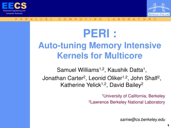
Auto-tuning Memory Intensive Kernels for Multicore Sam Williams SWWilliams@lbl.gov
Outline Challenges arising from Optimizing Single Thread Performance New Challenges Arising when Optimizing Multicore SMP Performance Performance Modeling and Little’s Law Multicore SMPs of Interest Auto-tuning Sparse Matrix-Vector Multiplication (SpMV) Auto-tuning Lattice-Boltzmann Magneto-Hydrodynamics (LBMHD) Summary
Instruction-Level Parallelism • On modern pipelined architectures, operations (like floating-point addition) have a latency of 4-6 cycles (until the result is ready). • However, independent adds can be pipelined one after another. • Although this increases the peak flop rate, • one can only achieve peak flops on the condition that on any given cycle the program has >4 independent adds ready to execute. • failing to do so will result in a >4x drop in performance. • The problem is exacerbated by superscalar or VLIW architectures like POWER or Itanium. • One must often reorganize kernels to express more instruction-level parallelism
ILP Example (1x1 BCSR) • Consider the core of SpMV • No ILP in the inner loop • OOO can’t accelerate serial FMAs time = time = time = time = time = 0 16 8 12 4 1x1 Register Block FMA FMA FMA FMA FMA for(all rows){ y0 = 0.0; for(all tiles in this row){ y0+=V[i]*X[C[i]] } y[r] = y0; }
ILP Example (1x4 BCSR) • What about 1x4 BCSR ? • Still no ILP in the inner loop • FMAs are still dependent on each other time = time = time = time = 0 4 8 12 1x4 Register Block FMA FMA FMA FMA for(all rows){ y0 = 0.0; for(all tiles in this row){ y0+=V[i ]*X[C[i] ] y0+=V[i+1]*X[C[i]+1] y0+=V[i+2]*X[C[i]+2] y0+=V[i+3]*X[C[i]+3] } y[r] = y0; }
ILP Example (4x1 BCSR) • What about 4x1 BCSR ? • Updating 4 different rows • The 4 FMAs are independent • Thus they can be pipelined. time = time = time = time = time = time = time = time = 7 0 2 1 3 4 5 6 4x1 Register Block FMA FMA FMA FMA FMA FMA FMA FMA for(all rows){ y0 = 0.0;y1 = 0.0; y2 = 0.0;y3 = 0.0; for(all tiles in this row){ y0+=V[i ]*X[C[i]] y1+=V[i+1]*X[C[i]] y2+=V[i+2]*X[C[i]] y3+=V[i+3]*X[C[i]] } y[r+0] = y0; y[r+1] = y1; y[r+2] = y2; y[r+3] = y3; }
Data-level Parallelism + + + + DLP = apply the same operation to multiple independent operands. Today, rather than relying on superscalar issue, many architectures have adopted SIMD as an efficient means of boosting peak performance. (SSE, Double Hummer, AltiVec, Cell, GPUs, etc…) Typically these instructions operate on four single precision (or two double precision) numbers at a time. However, some are more GPUs(32), Larrabee(16), and AVX(8) Failing to use these instructions may cause a 2-32x drop in performance Unfortunately, most compilers utterly fail to generate these instructions.
Memory-Level Parallelism (1) • Although caches may filter many memory requests, in HPC many memory references will still go all the way to DRAM. • Memory latency (as measured in core cycles) grew by an order of magnitude in the 90’s • Today, the latency of a memory operation can exceed 200 cycles (1 double every 80ns is unacceptably slow). • Like ILP, we wish to pipeline requests to DRAM • Several solutions exist today • HW stream prefetchers • HW Multithreading (e.g. hyperthreading) • SW line prefetch • DMA
Memory-Level Parallelism (2) HW stream prefetchers are by far the easiest to implement and exploit. They detect a series of consecutive cache misses and speculate that the next addresses in the series will be needed. They then prefetch that data into the cache or a dedicated buffer. To effectively exploit a HW prefetcher, ensure your array references accesses 100’s of consecutive addresses. e.g. read A[i]…A[i+255] without any jumps or discontinuities This force limits the effectiveness (shape) of the cache blocking you implemented in HW1 as you accessed: A[(j+0)*N+i]…A[(j+0)*N+i+B], jump A[(j+1)*N+i]…A[(j+1)*N+i+B], jump A[(j+2)*N+i]…A[(j+2)*N+i+B], jump …
Branch Misprediction A mispredicted branch can stall subsequent instructions by ~10 cycles. Select a loop structure that maximizes the loop length (keeps mispredicted branches per instruction to a minimum) Some architectures support predication either in hardware or software to eliminate branches (transforms control dependencies into data dependencies)
Cache Subtleties Set associative caches have a limited number of sets (S) and ways (W), the product of which is the capacity (in cache lines). As seen in HW1, it can be beneficial to reorganize kernels to reduce the working size and eliminate capacity misses. Conflict misses can severely impair performance, be very challenging to identify and eliminate. Given address may only be placed in W different locations in the cache. Poor access patterns or roughly power of two problem sizes can be especially bad Results in too many addresses mapped to the same set. Not all of them can be kept in the cache and some will have to be evicted. Padding arrays (problem sizes) or skewing access pattern can eliminate conflict misses.
Array padding Example Padding changes the data layout Consider a large matrix with a power of two number of double A[N][M];// column major with M~pow2 A[i][j] and A[i+1][j] will likely be mapped to the same set. We can pad each column with a couple extra rows double A[N][M+pad]; Such techniques are applicable in many other domains (stencils, lattice-boltzman methods, etc…)
New Challenges Arising whenOptimizing Multicore SMP Performance
What are SMPs ? • SMP = shared memory parallel. • Multiple chips (typically < 32 threads) can address any location in a large shared memory through a network or bus • Caches are almost universally coherent • You can still run MPI on an SMP, but • you trade free (always pay for it) cache-coherency traffic for additional memory traffic (for explicit communication) • you trade user-level function calls for system calls • Alternately, you use a SPMD threading model (pthreads, OpenMP, UPC) • If communication between cores or threads is significant, then threaded implementations win out. • As computation:communication ratio increases, MPI asymptotically approached threaded implementations.
What is multicore ?What are multicore SMPs ? • Today, multiple cores are integrated on the same chip • Almost universally this is done in a SMP fashion • For “convince”, programming multicore SMPs is indistinguishable from programming multi-socket SMPs. (easy transition) • Multiple cores can share: • memory controllers • caches • occasionally FPUs • Although there was a graceful transition from multiple sockets to multiple cores from the point of view of correctness, achieving good performance can be incredibly challenging.
Affinity 0 2 4 6 1 3 5 7 0 2 3 4 1 5 6 7 • We may wish one pair of threads to share a cache, but be disjoint from another pair of threads. • We can control the mapping of threads to linux processors via • #include<sched.h> + sched_set/getaffinity() • But, mapping of linux processors to physical cores/sockets is machine/OS dependent. • Inspect /proc/cpuinfo or use PLPA
NUMA Challenges Recent multicore SMPs have integrated the memory controllers on chip. As a result, memory-access is non-uniform (NUMA) That is, the bandwidth to read a given address varies dramatically among between cores Exploit NUMA (affinity+first touch) when you malloc/init data. Concept is similar to data decomposition for distributed memory
Implicit allocation for NUMA Consider an OpenMP example for implicitly NUMA initialization: #pragma omp parallel for for (j=0; j<N; j++) { a[j] = 1.0; b[j] = 2.0; c[j] = 0.0; } The first accesses to the array (read or write) must be parallelized. DO NOT TOUCH BETWEEN MALLOC AND INIT When the for loop is parallelized, each thread initializes a range of i Exploits the OS’s first touch policy. Relies on assumption OpenMP maps threads correctly
New Cache Challenges shared caches + SPMD programming models can exacerbate conflict misses. Individually, threads may produce significant cache associativity pressure based on access pattern. (power of 2 problem sizes) Collectively, threads may produce excessive cache associativity pressure. (power of 2 problem sizes decomposed with a power of two number of threads) This can be much harder to diagnose and correct This problem arises whether using MPI or a threaded model.
New Memory Challenges • The number of memory controllers and bandwidth on multicore SMPs is growing much slower than the number of cores. • codes are becoming increasingly memory-bound as a fraction of the cores can saturate a socket’s memory bandwidth • Multicore has traded bit-or word-parallelism for thread-parallelism. • However, main memory is still built from bit-parallel devices (DIMMs) • Must restructure memory-intensive apps to the bit-parallel nature of DIMMs (sequential access)
Synchronization Using multiple concurrent threads can create ordering and race errors. Locks are one solution. Must balance granularity and frequency SPMD programming model + barriers are often a better/simpler solution. spin barriers can be orders of magnitude faster than pthread library barriers. (Rajesh Nishtala, HotPar’09)
System Abstraction DRAM Cache RF CPU core FU’s • Abstractly describe any system (or subsystem) as a combination of black-boxed storage, computational units, and the bandwidth between them. • These can be hierarchically composed. • A volume of data must be transferred from the storage component, processed, and another volume of data must be returned. • Consider the basic parameters governing performance of the channel: Bandwidth, Latency, Concurrency • Bandwidth can be measured in: GB/s, Gflop/s, MIPS, etc… • Latency can be measured in: seconds, cycles, etc… • Concurrency the volume in flight across the channel, and can be measured in bytes, cache lines, operations, instructions, etc…
Little’s Law Concurrencyexpressed / Latency BWattained = min BWmax • Little’s law related concurrency, bandwidth, and latency • To achieve peak bandwidth, one must satisfy: • Concurrency = Latency × Bandwidth • For example, a memory controller with 20GB/s of bandwidth, and 100ns of latency requires the CPU to express 2KB of concurrency • (memory-level parallelism) • Similarly, given an expressed concurrency, one can bound attained performance: • That is, as more concurrency is injected, we get progressively better performance • Note, this assumes continual, pipelined accesses.
Where’s the bottleneck? DRAM Cache RF CPU core FU’s • We’ve described bandwidths • DRAM CPU • Cache Core • Register File Functional units • But in an application, one of these may be a performance-limiting bottleneck. • We can take any pair and compare how quickly data can be transferred to how quickly it can be processed to determine the bottleneck.
Arithmetic Intensity • Consider the first case (DRAM-CPU) • True Arithmetic Intensity (AI) ~ Total Flops / Total DRAM Bytes • Some HPC kernels have an arithmetic intensity that scales with problem size (increased temporal locality), but remains constant on others • Arithmetic intensity is ultimately limited by compulsory traffic • Arithmetic intensity is diminished by conflict or capacity misses. O( log(N) ) O( 1 ) O( N ) A r i t h m e t i c I n t e n s i t y SpMV, BLAS1,2 FFTs Stencils (PDEs) Dense Linear Algebra (BLAS3) Lattice Methods Particle Methods
Kernel Arithmetic Intensityand Architecture • For a given architecture, one may calculate its flop:byte ratio. • For a 2.3GHz Quad Core Opteron, • 1 SIMD add + 1 SIMD multiply per cycle per core • 12.8GB/s of DRAM bandwidth • = 36.8 / 12.8 ~ 2.9 flops per byte • When a kernel’s arithmetic intensity is substantially less than the architecture’s flop:byte ratio, transferring data will take longer than computing on it memory-bound • When a kernel’s arithmetic intensity is substantially greater than the architecture’s flop:byte ratio, computation will take longer than data transfers compute-bound
Memory Traffic Definition • Total bytes to/from DRAM • Can categorize into: • Compulsory misses • Capacity misses • Conflict misses • Write allocations • … • Oblivious of lack of sub-cache line spatial locality
Roofline ModelBasic Concept Attainable Performanceij = min FLOP/s with Optimizations1-i AI * Bandwidth with Optimizations1-j • Synthesize communication, computation, and locality into a single visually-intuitive performance figure using bound and bottleneck analysis. • where optimization i can be SIMDize, or unroll, or SW prefetch, … • Given a kernel’s arithmetic intensity (based on DRAM traffic after being filtered by the cache), programmers can inspect the figure, and bound performance. • Moreover, provides insights as to which optimizations will potentially be beneficial.
Roofline ModelBasic Concept 256.0 128.0 64.0 32.0 16.0 8.0 4.0 2.0 1.0 0.5 1/8 1/4 1/2 1 2 4 8 16 • Plot on log-log scale • Given AI, we can easily bound performance • But architectures are much more complicated • We will bound performance as we eliminate specific forms of in-core parallelism Opteron 2356 (Barcelona) peak DP attainable GFLOP/s Stream Bandwidth actual FLOP:Byte ratio
Roofline Modelcomputational ceilings 256.0 128.0 64.0 32.0 16.0 8.0 4.0 2.0 1.0 0.5 1/8 1/4 1/2 1 2 4 8 16 • Opterons have dedicated multipliers and adders. • If the code is dominated by adds, then attainable performance is half of peak. • We call these Ceilings • They act like constraints on performance Opteron 2356 (Barcelona) peak DP mul / add imbalance attainable GFLOP/s Stream Bandwidth actual FLOP:Byte ratio
Roofline Modelcomputational ceilings 256.0 128.0 64.0 32.0 16.0 8.0 4.0 2.0 1.0 0.5 1/8 1/4 1/2 1 2 4 8 16 • Opterons have 128-bit datapaths. • If instructions aren’t SIMDized, attainable performance will be halved Opteron 2356 (Barcelona) peak DP mul / add imbalance attainable GFLOP/s w/out SIMD Stream Bandwidth actual FLOP:Byte ratio
Roofline Modelcomputational ceilings 256.0 128.0 64.0 32.0 16.0 8.0 4.0 2.0 1.0 0.5 1/8 1/4 1/2 1 2 4 8 16 • On Opterons, floating-point instructions have a 4 cycle latency. • If we don’t express 4-way ILP, performance will drop by as much as 4x Opteron 2356 (Barcelona) peak DP mul / add imbalance attainable GFLOP/s w/out SIMD Stream Bandwidth w/out ILP actual FLOP:Byte ratio
Roofline Modelcommunication ceilings 256.0 128.0 64.0 32.0 16.0 8.0 4.0 2.0 1.0 0.5 1/8 1/4 1/2 1 2 4 8 16 • We can perform a similar exercise taking away parallelism from the memory subsystem Opteron 2356 (Barcelona) peak DP attainable GFLOP/s Stream Bandwidth actual FLOP:Byte ratio
Roofline Modelcommunication ceilings 256.0 128.0 64.0 32.0 16.0 8.0 4.0 2.0 1.0 0.5 1/8 1/4 1/2 1 2 4 8 16 • Explicit software prefetch instructions are required to achieve peak bandwidth Opteron 2356 (Barcelona) peak DP attainable GFLOP/s Stream Bandwidth w/out SW prefetch actual FLOP:Byte ratio
Roofline Modelcommunication ceilings 256.0 128.0 64.0 32.0 16.0 8.0 4.0 2.0 1.0 0.5 1/8 1/4 1/2 1 2 4 8 16 • Opterons are NUMA • As such memory traffic must be correctly balanced among the two sockets to achieve good Stream bandwidth. • We could continue this by examining strided or random memory access patterns Opteron 2356 (Barcelona) peak DP attainable GFLOP/s Stream Bandwidth w/out SW prefetch w/out NUMA actual FLOP:Byte ratio
Roofline Modelcomputation + communication ceilings 256.0 128.0 64.0 32.0 16.0 8.0 4.0 2.0 1.0 0.5 1/8 1/4 1/2 1 2 4 8 16 • We may bound performance based on the combination of expressed in-core parallelism and attained bandwidth. Opteron 2356 (Barcelona) peak DP mul / add imbalance attainable GFLOP/s w/out SIMD Stream Bandwidth w/out SW prefetch w/out NUMA w/out ILP actual FLOP:Byte ratio
Roofline Modellocality walls 256.0 128.0 64.0 32.0 16.0 8.0 4.0 2.0 1.0 0.5 1/8 1/4 1/2 1 2 4 8 16 • Remember, memory traffic includes more than just compulsory misses. • As such, actual arithmetic intensity may be substantially lower. • Walls are unique to the architecture-kernel combination Opteron 2356 (Barcelona) peak DP mul / add imbalance attainable GFLOP/s w/out SIMD Stream Bandwidth w/out SW prefetch w/out NUMA only compulsory miss traffic w/out ILP FLOPs AI = Compulsory Misses actual FLOP:Byte ratio
Roofline Modellocality walls 256.0 128.0 64.0 32.0 16.0 8.0 4.0 2.0 1.0 0.5 1/8 1/4 1/2 1 2 4 8 16 • Remember, memory traffic includes more than just compulsory misses. • As such, actual arithmetic intensity may be substantially lower. • Walls are unique to the architecture-kernel combination Opteron 2356 (Barcelona) peak DP mul / add imbalance attainable GFLOP/s w/out SIMD Stream Bandwidth w/out SW prefetch w/out NUMA +write allocation traffic only compulsory miss traffic w/out ILP FLOPs AI = Allocations + Compulsory Misses actual FLOP:Byte ratio
Roofline Modellocality walls 256.0 128.0 64.0 32.0 16.0 8.0 4.0 2.0 1.0 0.5 1/8 1/4 1/2 1 2 4 8 16 • Remember, memory traffic includes more than just compulsory misses. • As such, actual arithmetic intensity may be substantially lower. • Walls are unique to the architecture-kernel combination Opteron 2356 (Barcelona) peak DP mul / add imbalance attainable GFLOP/s w/out SIMD Stream Bandwidth w/out SW prefetch w/out NUMA +capacity miss traffic +write allocation traffic only compulsory miss traffic w/out ILP FLOPs AI = Capacity + Allocations + Compulsory actual FLOP:Byte ratio
Roofline Modellocality walls 256.0 128.0 64.0 32.0 16.0 8.0 4.0 2.0 1.0 0.5 1/8 1/4 1/2 1 2 4 8 16 • Remember, memory traffic includes more than just compulsory misses. • As such, actual arithmetic intensity may be substantially lower. • Walls are unique to the architecture-kernel combination Opteron 2356 (Barcelona) peak DP mul / add imbalance attainable GFLOP/s w/out SIMD Stream Bandwidth w/out SW prefetch w/out NUMA +conflict miss traffic +capacity miss traffic +write allocation traffic only compulsory miss traffic w/out ILP FLOPs AI = Conflict + Capacity + Allocations + Compulsory actual FLOP:Byte ratio
Optimization Categorization Maximizing (attained) In-core Performance Maximizing (attained) Memory Bandwidth Minimizing (total) Memory Traffic
Optimization Categorization Maximizing In-core Performance Maximizing Memory Bandwidth Minimizing Memory Traffic • Exploit in-core parallelism • (ILP, DLP, etc…) • Good (enough) • floating-point balance
Optimization Categorization Maximizing In-core Performance Maximizing Memory Bandwidth Minimizing Memory Traffic • Exploit in-core parallelism • (ILP, DLP, etc…) • Good (enough) • floating-point balance ? reorder ? unroll & jam ? eliminate branches ? explicit SIMD
Optimization Categorization TLB blocking unit-stride streams ? DMA lists ? SW prefetch ? memory affinity ? ? Maximizing In-core Performance Maximizing Memory Bandwidth Minimizing Memory Traffic • Exploit in-core parallelism • (ILP, DLP, etc…) • Good (enough) • floating-point balance • Exploit NUMA • Hide memory latency • Satisfy Little’s Law reorder ? unroll & jam ? eliminate branches ? explicit SIMD ?
Optimization Categorization TLB blocking unit-stride streams ? DMA lists ? SW prefetch ? memory affinity ? ? Maximizing In-core Performance Maximizing Memory Bandwidth Minimizing Memory Traffic • Exploit in-core parallelism • (ILP, DLP, etc…) • Good (enough) • floating-point balance • Exploit NUMA • Hide memory latency • Satisfy Little’s Law • Eliminate: • Capacity misses • Conflict misses • Compulsory misses • Write allocate behavior reorder ? ? cache blocking unroll & jam ? ? array padding ? eliminate branches ? streaming stores explicit SIMD ? compress data ?
Optimization Categorization ? memory affinity ? SW prefetch ? DMA lists ? unit-stride streams ? TLB blocking Maximizing In-core Performance Maximizing Memory Bandwidth Minimizing Memory Traffic • Exploit in-core parallelism • (ILP, DLP, etc…) • Good (enough) • floating-point balance • Exploit NUMA • Hide memory latency • Satisfy Little’s Law • Eliminate: • Capacity misses • Conflict misses • Compulsory misses • Write allocate behavior ? reorder ? cache blocking ? unroll & jam ? array padding ? eliminate branches ? streaming stores ? explicit SIMD ? compress data
Roofline Modellocality walls 256.0 128.0 64.0 32.0 16.0 8.0 4.0 2.0 1.0 0.5 1/8 1/4 1/2 1 2 4 8 16 • Optimizations remove these walls and ceilings which act to constrain performance. Opteron 2356 (Barcelona) peak DP mul / add imbalance attainable GFLOP/s w/out SIMD Stream Bandwidth w/out SW prefetch w/out NUMA +conflict miss traffic +capacity miss traffic +write allocation traffic only compulsory miss traffic w/out ILP actual FLOP:Byte ratio
Roofline Modellocality walls 256.0 128.0 64.0 32.0 16.0 8.0 4.0 2.0 1.0 0.5 1/8 1/4 1/2 1 2 4 8 16 • Optimizations remove these walls and ceilings which act to constrain performance. Opteron 2356 (Barcelona) peak DP mul / add imbalance attainable GFLOP/s w/out SIMD Stream Bandwidth w/out SW prefetch w/out NUMA only compulsory miss traffic w/out ILP actual FLOP:Byte ratio