Download
1 / 33
330 likes | 333 Views
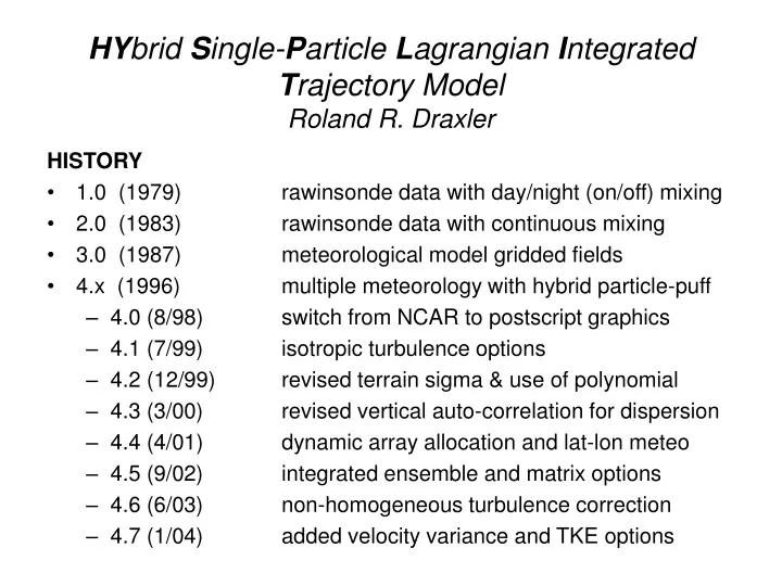
HY brid S ingle- P article L agrangian I ntegrated T rajectory Model Roland R. Draxler. HISTORY 1.0 (1979) rawinsonde data with day/night (on/off) mixing 2.0 (1983) rawinsonde data with continuous mixing 3.0 (1987) meteorological model gridded fields

E N D
HYbrid Single-Particle Lagrangian Integrated Trajectory ModelRoland R. Draxler HISTORY • 1.0 (1979) rawinsonde data with day/night (on/off) mixing • 2.0 (1983) rawinsonde data with continuous mixing • 3.0 (1987) meteorological model gridded fields • 4.x (1996) multiple meteorology with hybrid particle-puff • 4.0 (8/98) switch from NCAR to postscript graphics • 4.1 (7/99) isotropic turbulence options • 4.2 (12/99) revised terrain sigma & use of polynomial • 4.3 (3/00) revised vertical auto-correlation for dispersion • 4.4 (4/01) dynamic array allocation and lat-lon meteo • 4.5 (9/02) integrated ensemble and matrix options • 4.6 (6/03) non-homogeneous turbulence correction • 4.7 (1/04) added velocity variance and TKE options
Overview of Model Features • Predictor-corrector advection scheme • Linear spatial & temporal interpolation of meteorology from external sources • Vertical mixing based upon SL similarity, BL Ri, or TKE • Horizontal mixing based upon velocity deformation, SL similarity, or TKE • Puff and Particle dispersion computed from velocity variances • Concentrations from particles-in-cell, or Puffs with Top-Hat or Gaussian distributions • Multiple simultaneous meteorology and / or concentration grids
Eulerian Dispersion Models • Advection-Diffusion Equation • Solve for local derivative • at all grid points • Dispersion a function of concentration gradients • Handles many sources • complex chemistry • Artificial diffusion can be a problem for point sources
Lagrangian Dispersion Models • Solve for total derivative • along the trajectory • Computation required only at nearby grid points • Concentrations for point sources handled correctly • Implicit linearity • Concentration at a receptor the sum from all sources • Solution for too many sources can be inefficient
Relationship of Trajectory to Height FieldAnimation Example • July 12-13, 1979 • 700 hPa height field • Snapshots 4x / day • Trajectory follows height • Isobaric calculation • Parcel release at 3 km • Represents advection of point integrated in space and time!
Equations for the Trajectory Computation • Position computed from average velocity at the initial position (P) and first-guess position (P') • P(t+dt) = P(t) + 0.5 [ V(P,t) + V(P',t+dt) ] dt • P'(t+dt) = P(t) + V(P,t) dt • The integration time step is variable: Vmax dt < 0.75 • The meteorological data remain on its native horizontal coordinate system • Meteorological data are interpolated to an internal terrain-following (s) vertical coordinate system • s = (Ztop - Zmsl) / (Ztop - Zgl)
Example Trajectory Graphic from HYSPLIT • Postscript output format • Labels describe • Starting time • Starting location • Starting height • Meteorological data • Vertical Projection • Shown by time • Height or pressure
Example of Numerical Trajectory Error • The numerical accuracy of the computation can be estimated by running a forward and then backward trajectory to the origin point • The numerical integration errors will be much smaller than the data representation errors
Example of Meteorological Data Errors • The largest source of error is the representation of variables by discrete data points • A qualitative measure of the error can be determined by running trajectories using meteorological data from different sources • Trajectories have been computed using data from ECMWF, NOAA, and MM5 (108and 36-km) • Differences between trajectories are much greater than the numerical error
Ensemble Estimates of Trajectory Error • Each member of the trajectory ensemble is calculated by offsetting the meteorological data by a fixed grid factor • The default offset is one meteorological grid point in the horizontal and 0.01 sigma units in the vertical • The results in 27 members for all-possible offsets in X, Y, Z
Trajectory Representation of a Plume • A single trajectory cannot properly represent the growth of a pollutant cloud when the wind field varies in space and height • The simulation must be conducted using many pollutant particles • New trajectories are started every 4-h at 10, 100, and 200 m AGL to represent the boundary layer transport
Dispersive 2500 Particle Plume Simulation • Particle: a point mass of contaminant. A fixed number is released with mean and random motion. • Puff: a 3-D cylinder with a growing concentration distribution in the vertical and horizontal. Puffs may split if they become too large. • Hybrid: a circular 2-D object (planar mass, having zero depth), in which the horizontal contaminant has a “puff” distribution and in the vertical functions as a particle.
Particle and Puff Distribution after 24-hRandom Particles (left) and Mean Puff Positions (right) X(t+dt)=Xmean(t+dt)+U'(t+dt) dt U'(t+dt)=R(dt) U'(t)+U" (1-R(dt)2 )0.5 R(dt)=exp(-dt/TLx) U“ = s x [Gaussian Random Number] sh2 = (Xi-Xm)2 dsh/dt = 20.5 su su = (Kx / TL)0.5
Particle Positions with Dispersion • Initial release 1000 particles • Each advection step computed with mean wind and turbulence • Position results after 24 hrs • Horizontal distribution primarily due differential advection • Effects of horizontal and vertical wind shear as particles mix to different levels
Computation of Air Concentration • Each particle is assigned a pollutant mass • Concentration is simply the mass sum / volume • Volume may be defined as the … • concentration grid cell for particles • the volumetric distribution of the puff 3D particle: dC = q (dx dy dz)-1 Hybrid Top-Hat: dC = q (pi r2 dz)-1 Hybrid Gaussian: dC = q (2 pi s2 dz)–1 exp(-x2 / 2s2) Puff Top Hat: dC = q (pi r2 dzp)-1 Puff Gaussian: dC = q (2 pi s2 dzp)–1 exp(-x2 / 2s2)
Concentrations Resulting from a Single Particle • Concentration Grid defined at 50 km resolution • Air concentration = unit mass / volume • Concentration depends on particle’s residence time in cell • A single particle (or trajectory) cannot represent the complex plume
Concentrations Resulting from the Release of 1000 Particles and 50-km Grid • Results shown after 24 hours • 50 km concentration grid size • The internal plume structure is is not well resolved due to the large concentration cell size
Concentrations Resulting from the Release of 1000 Particles and 25-km Grid • Shown after 24 hours • 25 km concentration cell size • Smaller cell sizes shows more structure • Horizontal distribution appears to be noisy • Needs more particles • Suggests use of puff approach • Faster to model growth of particle distribution (puff)
Why Puff Dispersion? • Simulation models the growth of the particle distribution (standard deviation) • Requires fewer particles (puffs) • Growth uses the same turbulence parameters • Hybrid method suggested default • Fewer puffs required for horizontal distribution • Vertical shears captured more accurately by particles
Turbulence Options • Standard Diffusivity / Deformation • Kz = k wh z (1 - z/Zi) • Kh = 2-0.5 (c d)2 |du/dy + dv/dx| • Velocity Variances for Short-Range • w’2 = 3.0 u*2 (1 – z/zi)3/2 • u’2 = 4.0 u*2 (1 – z/zi)3/2 • v’2 = 4.5 u*2 (1 – z/zi)3/2 • Turbulent Kinetic Energy • E = 0.5 (u’2 + v’2 + w’2) • w’2 =0.52 E, u’2 =0.70 E, v’2 =0.78 E • u’2 = v’2 = 0.36 w*2
Horizontal Distribution for a Single Puff Top-Hat Distribution Uniform over 1.54 sigma Mean = Gaussian Gaussian Distribution Shown over 3 sigma Mean = Top Hat
Horizontal Distribution for 500 Puffs Left side using the Top-Hat Central region identical to the Gaussian Sharp transition at the edges Right side using the Gaussian Central region identical to Top-Hat Smooth transition at the edges
Example 24-h Average Air ConcentrationsUsing 500 top-hat particle-puffs Actual grid cell values Standard display output Uses grid smoothing to produce cleaner contours
Ensemble ConcentrationsProbability of Exceeding 10-12 • NCEP/NCAR • ECMWF ERA40 • MM5 (108, 36, 12, 4 km) Internal grid shift 27 member ensemble Using 36-km MM5
Ensemble Calculation Example from ANATEX • Plot shows 90th percentile model concentration contours for a 24h period several days after the tracer release • Within a contour, 10% of the members predict a higher concentration and outside of the contour 90% of the members predict a lower concentration • Locations for the measured values are indicated by X and the corresponding value
Local Scale VerificationWashington D.C. - Metropolitan Tracer Experiment • Tracer releases • Rockville, Mt. Vernon, Lorton • every 36-h at 2 locations • Sampling • 3 locations at 8-h • 93 locations monthly • Duration all 1984 • Meteorology • ECMWF ERA-40 (shown) • MM5 4-km (incomplete) • Nocturnal intensives • Plume measurements • Tethersonde data
Regional Scale VerificationIdaho Forest Fires August 2000 • Daily particle snapshot positions at 1800 UTC • Squares represent TOMS satellite aerosol index value • Continuous particle release to correspond with with major forest fire location • Particles line up with air mass boundaries
Continental Scale VerificationChina Dust Storm April 2001 • Emissions using integrated PM10 module • Friction velocity over desert land-use grid cells exceeds threshold velocity • Daily particle snapshot positions at 0600 UTC • Colored squares show TOMS aerosol index value
China April 2001 Dust Storm PM10 Concentrations • Predicted concentrations over the US 10 to 18 days after the event started • Slight over-prediction at most sites due to no-deposition during simulation • Arrival times match measured times • Measurements are 24h averages taken every 3rd day
China 2002 Dust Storm PM10 • March 2002 event not global like the April 2001 dust storm • Hourly PM10 measurements shown in Seoul, Korea • Excellent match with time of onset and peak concentrations • Measured duration much greater, probably due to particle re-suspension • As in other cases, model predicts emission locations and amount
Quantitative VerificationStatistics for Several Long-Range Experiments Experiment Model R FB FMS KS RANK ACURATE May 2002 0.25 -0.05 18.73 79 1.43 Dec 2002 0.25 +0.48 18.01 79 1.21 ANATEX1 Dec 2002 0.34 0.29 35.09 59 1.73 Dec 2003 0.44 0.18 32.84 59 1.85 ANATEX2 Dec 2002 0.18 0.16 34.06 56 1.73 Dec 2003 0.18 0.19 33.97 56 1.72 ANATEX3 Dec 2002 0.14 0.12 21.01 50 1.67 Dec 2003 0.17 0.0 20.70 56 1.73 CAPTEX Dec 2002 0.00 -0.12 16.78 71 1.40 Dec 2003 0.02 -0.27 17.07 71 1.33 INEL74 Apr 2001 0.00 0.13 7.97 92 0.48 Dec 2002 0.00 1.39 7.27 92 0.46 OKC80 Dec 2002 0.08 -0.66 27.60 34 1.52 Dec 2003 0.43 -0.87 35.01 43 1.67 ETEX Apr 2001 0.48 0.33 57.27 68 1.96 Dec 2003 0.45 0.78 47.69 68 1.61
Averaged Verification Statistics Temporally Averaged Verification Statistics for Long-Range Experimental Data Experi Experiment Model R FB FMS KS RANK ACURATE May 2002 0.90 -0.06 100.0 58 3.20 Dec 2002 0.86 +0.47 100.0 78 2.73 ANATEX1 Dec 2002 0.85 0.26 100.0 18 3.41 Dec 2003 0.85 0.14 100.0 23 3.43 ANATEX2 Dec 2002 0.56 0.13 100.0 26 2.98 Dec 2003 0.48 0.16 100.0 26 2.89 ANATEX3 Dec 2002 0.25 0.05 98.67 48 2.54 Dec 2003 0.20 -.06 98.67 46 2.54 CAPTEX Dec 2002 0.80 -0.17 94.87 17 3.33 Dec 2003 0.76 -0.31 94.87 19 3.18 INEL74 Apr 2001 0.13 1.39 100.0 89 1.43 Dec 2002 0.35 1.41 100.0 98 1.44 OKC80 Dec 2002 0.96 -0.64 80.0 18 3.21 Dec 2003 0.83 -0.85 90.0 20 2.97 ETEX Apr 2001 0.51 0.23 84.89 20 2.79 Dec 2003 0.59 0.65 82.55 20 2.65
Summary • Point source pollutant transport and dispersion calculations are very sensitive to source-receptor geometry and the meteorological data driving the calculation • Event based verification includes all the above limitations of temporal and spatial resolution • Future systems should incorporate automated verification linked with satellite observations of smoke from fires and dust storms