Download
1 / 15
150 likes | 372 Views
Chapter 3 Cost-Volume-Profit Analysis. Cost-Volume-Profit Analysis. Examines the behaviour of total revenues, total costs, and operating income as changes occur in the output level, selling price, variable costs, or fixed costs Assumptions of CVP Analysis

E N D
Cost-Volume-Profit Analysis • Examines the behaviour of total revenues, total costs, and operating income as changes occur in the output level, selling price, variable costs, or fixed costs Assumptions of CVP Analysis • Revenues change in relation to production and sales • Costs can be divided in variable and fixed categories • Revenues and costs behave in a linear fashion • Costs and prices are known • If more than one product exists, the sales mix is constant • We can ignore the time value of money Page 67
Total for Per Unit 2 units % Revenue $200 $400 100% Variable costs 12024060% Contribution margin $80 $160 40% Contribution Margin • Contribution margin is equal to the difference between total revenue and total variable costs Contribution margin per unit = Selling price – Variable cost per unit Contribution margin percentage = Contribution margin per unit / Selling price per unit Pages 68 - 69
Contribution Margin Income Statement • Income statement that groups line items by cost behaviour to highlight the contribution margin Packages Sold 0 1 2 25 40 Revenue $0 $200 $400 $5,000 $8,000 Variable costs 0 120 240 3,000 4,800 Contribution margin 0 80 160 2,000 3,200 Fixed costs 2,000 2,000 2,000 2,000 2,000 Operating income $(2,000) $(1,920) $(1,840) $0 $1,200 Page 69
Breakeven Point • Quantity of output where total revenues equal total costs • Point where operating income equals zero Breakeven point in units = Fixed costs / Contribution margin per unit = $2,000 / $80 = 25 units Breakeven point in dollars = Fixed costs / Contribution margin % = $2,000 / 40% = $5,000 Page 71
Cost-Volume-Profit Graph $10,000 $8,000 $6,000 $4,000 $2,000 $0 Total revenues line Breakeven Point 25 units Total costs line Operating income Operating loss 0 10 20 30 40 50 Units Sold Page 72
Target Operating Income • For most firms in the private sector, the main objective is not to break even • Convert after-tax desired net income to its before-tax equivalent operating income Target operating income = Target net income / (1 - tax rate) Target Unit Sales = (Fixed costs + Target operating income) / Contribution margin per unit Target Dollar Sales = (Fixed costs + Target operating income) / Contribution margin % Pages 73 - 75
Sensitivity Analysis • Sensitivity analysis is a “what-if” technique that examines how a result will change if the original predicted data are not achieved or if an underlying assumption changes • What will happen to operating income if volume declines by 5%? • What will happen to operating income if variable costs increase by 10% per unit? • Sensitivity analysis broadens management’s perspectives about possible outcomes Pages 76 - 77
Option 2 $1,400 Fixed Fee + 5% Commission Option 1 $2,000 Fixed Fee Option 3 20% Commission Rev Rev Rev $ $ $ Cost Cost Cost Units Units Units Breakeven = 25 units Breakeven = 20 units Breakeven = 0 units Alternative Cost Structures • CVP helps managers assess the risks and potential benefits of adopting alternative cost structures Example: Alternative rental arrangements Pages 77 - 78
Revenue Mix • Revenue mix (or sales mix) is the relative combination of quantities of products or services that make up total revenue • Sales mix of Do-All : Superword = 2 : 1 Breakeven point in units = 30 units 20 units of Do-All 10 units of Superword Do-All Do-All Superword Pages 73 - 75
Multiple Cost Drivers • In many cases there may be multiple cost drivers Do-All Software Example Variable costs: $40 per software package sold $15 per invoice issued Operating income = Revenue – ($40 x Packages sold) – ($15 x Invoices issued) – Fixed costs • In cases where there are multiple cost drivers there are multiple breakeven points Pages 81 - 82
Contribution Margin & Gross Margin Merchandising Sector Contribution Margin Format Revenues $200 Variable costs: Cost of goods sold $120 Other variable 43 163 Contribution margin 37 Fixed costs: Cost of goods sold 5 Other fixed 19 24 Operating income $13 Gross Margin Format Revenues $200 Cost of goods sold (120+5) 125 Gross margin 75 Operating costs (43+19) 62 Operating income $13 Pages 82 - 83
Contribution Margin & Gross Margin Manufacturing Sector Contribution Margin Format Revenues $1,000 Variable costs: Manufacturing $250 Non-manufacturing 270 520 Contribution margin 480 Fixed costs: Manufacturing 160 Non-manufacturing 138 298 Operating income $182 Gross Margin Format Revenues $1,000 Cost of goods sold (250+160) 410 Gross margin 590 Non-manufacturing (270+138) 408 Operating income $182 Pages 81 - 82
Decision Models and Uncertainty • Managers make predictions and decisions in a world of uncertainty • Estimate events that are likely to occur and assign probabilities to each outcome • Probability distribution describes the likelihood of each mutually exclusive and collectively exhaustive set of events (must add to 1.00) • Expected value is a weighted average of the outcomes with the probability of each outcome serving as the weight Pages 86 - 87
Uncertainty Example Proposal A: Spy Novel 0.5 Probability 0.4 0.3 0.2 0.1 • 2 3 4 5 6 7 8 9 Cash Inflow ($000,000) Expected value = (0.1*$300,000) + (.02*$350,000) + (.04*$400,000) + (0.2*$450,000) + (0.1*$500,000) = $400,000 Page 87