Download
1 / 34
340 likes | 459 Views
Geographic Routing without Location Information. Yu-Min Tseng. Routing in Wireless Network. Distance vector DSDV On-demand DSR, TORA, AODV Discovers & caches routes on demand Geographic GPSR, DREAM, GRID GPSR – scales very well. What’s the problem?. No address aggregation

E N D
Geographic Routing without Location Information Yu-Min Tseng
Routing in Wireless Network • Distance vector • DSDV • On-demand • DSR, TORA, AODV • Discovers & caches routes on demand • Geographic • GPSR, DREAM, GRID • GPSR – scales very well
What’s the problem? • No address aggregation • Except geographic routing, all other approaches require O(N) state per node • Routing by coordinates is a good way to avoid O(N) per-node routing state
Why geographic routing without location information? • GPS takes power, doesn’t work indoors • Obstacles, no-ideal radios • Coordinates computed will reflect true connectivity & not the geographic locations of the nodes
Geographic routing • Choose coordinates for nodes • Greedy routing • Proceed closer to destination at each hop • How to deal with voids? • “Addresses” of nodes keep changing as they move • Need a lookup service for the current location of a node
Outline • Perimeter nodes & their locations are known • Perimeter nodes are known but their locations are not known • Nothing is known about the perimeter • Performance evaluation
Rubber Bands • Iterative process for picking coordinates for a node • Some nodes along with periphery of the network know their correct (relative) locations and are fixed • Other nodes compute coordinates by relaxation
Every node moves to the average of its neighbors coordinates at each step
Evaluation • Success Rate • Using purely greedy routing • Without dead-end avoidance techniques • Average Path Length • Average number of hops taken along the path
True geographic coordinate 3200 nodes uniformly spread, 64 perimeter nodes, Radio range is 8 unit. Each node have avg 16 neighbors.
Perimeter nodes are known (10 iterations) All non-perimeter nodes start with same initial coordinates
Perimeter nodes are known (1000 iterations) Success rate 0.993, average path length 17.1
True geographic coordinate Success rate 0.989, average path length 16.8
Resilience of rubber bands Success rate 0.99, average path length 17.1
Resilience of the rubber band Success rate 0.981, average path length 17.3
Rubber bands (cont’d) • We need a periodic heartbeat between neighbors so each node can maintain a list of its neighbors • We just send the current position of the node along with the heartbeat packet it broadcasts • Each time a heartbeat packet is received, we re-compute the coordinate
Outline • Perimeter nodes & their locations are known • Perimeter nodes are known but their locations are not known • Nothing is known about the perimeter • Performance evaluation
Perimeter coordinate algorithm • Perimeter coordinate algorithm • Perimeter nodes broadcast a HELLO message to network, discover the distance to all other perimeter node perimeter vector • Perimeter nodes broadcast their perimeter vector to network • Every perimeter node use a triangulation algorithm to compute the coordinates of all perimeter nodes • Perimeter nodes flood O(N2) overhead
Perimeter coordinate algorithm (cont’d) • Measured_dist(I, j) • Distance between node i & j in perimeter vector • Dist(I, j) • Geometric distance between the virtual coordinates of node I & j • For minimizing the potential energy consumed, make the coordinate proportional to the hop count distance
Bootstrapping beacons • Two designated bootstrap beacons flood with HELLO messages • Perimeter nodes compute coordinates with bootstrap nodes • Compute the center of gravity (CG) • CG forms the origin • First bootstrap node defines x axis • Second bootstrap node define y axis
After 1 iteration, success rate 0.992, average path length 17.2 After 10 iterations, success rate 0.994, average path length 17.2
Outline • Perimeter nodes & their locations are known • Perimeter nodes are known but their locations are not known • Nothing is known about the perimeter • Performance evaluation
Perimeter node criterion • If a node is the farthest away, among all its 2-hop neighbors from bootstrap nodes, then the node decides that it is on the perimeter • A designated bootstrap node periodically broadcasts, nodes periodically re-assess whether they lie on the perimeter or not • Need a leader election protocol to deal with failure of this bootstrap node • Overhead doesn’t depend on N
Coordinate projection on circle • Origin is the CG of perimeter nodes • Radius is the average distance of perimeter nodes from CG • Virtual circle makes it easier to support mobility • If a node concludes that it is on the perimeter, it projects itself on circle & stays fixed
After 10 iterations, success rate 0.996, average path length 17.3
Outline • Perimeter nodes & their locations are known • Perimeter nodes are known but their locations are not known • Nothing is known about the perimeter • Performance evaluation
Experiment design • Event driven packet level simulator • Doesn’t model application traffic or collisions • Scales to 3200 nodes with packet events & 12800 nodes without events • 3200 nodes distributed randomly in a 200x200 square. Radio range is 8, density is held constant while scaling up